User Guide — MAPP 3D
System design and prediction tool


Welcome to Meyer Sound Labs MAPP 3D User Guide. The user guide provides the information needed to create projects, along with reference materials.
Overview
MAPP 3D presents users with an intuitive interface to create 3D models of venues, add loudspeakers and microphones, and optimize a system design using Meyer Sound Labs products. This page provides detailed information about the MAPP 3D interface and functions.
Operating systems
MAPP 3D runs on the current versions of MacOS and Windows operating systems. Though it may operate on earlier operating system versions, proper operation has not been tested.
Video monitor display
MAPP 3D supports 1280×768 up to HD and Retina resolution displays. Higher resolutions may scale incorrectly or cause application instability. Please update graphics drivers to the latest version, which may enable 4k resolution.
Welcome window

Create an empty project
Open an existing project from a storage device
Activate/deactivate the MAPP 3D application
Open recent projects (lists recently opened/saved projects)
Open a template (displays available MAPP 3D project templates)
Click Choose after selecting a recent Project or Template. Click Cancel to close the application.
Project properties
When a new project is created, the Project Properties window is displayed. Basic information about the project and venue can be recorded here. This information is saved as part of the project file (.mapp).

Project Properties
Main application window

Inventory/Express Settings tabs
Inventory: View All selected; click icons
 to display only Geometry, Signal Processors, Loudspeaker Systems, or Microphones.
Express Settings: Use the drop-down menu at the top of the tab to select an object; displays the common properties for editing. For all object properties, use the Object Settings tab.
Generator Gain Level
Adjustment of signal level for all loudspeakers in model; affects SPL values.
Generator Signal Type
Pink Noise, B-Noise, or M-Noise; see definitions.
Pressure Map Settings
Select bandwidth, frequency range, and center frequency of prediction (SPL values valid only for bandwidth and frequency selected—use Headroom tab for broadband SPL).
Click Predict to generate an SPL/Attenuation map for any geometry that has been selected for prediction in the geometry’s Object Settings. Click Clear to remove all of the prediction data.
SPL Data
Displays Maximum and Minimum dBSPL(z-unweighted) and the SPL difference across selected prediction planes.
Power Calculation
Select to open the Amperage and BTU calculator at meyersound.com to calculate system current requirements and thermal dissipation.
Tools
Select, Pan, Orbit, Distance Tape Measure, Scale, Rotate, Align, Mirror, Zoom In, Zoom Out, Zoom to Extents, and Array.
Primitives/Modifiers Tabs
Primitives: select 2D/3D Primitive presets or Free Draw to add to model.
Modifiers: provides tools to modify 2D/3D Primitives.
Properties/Layers Tabs
Properties: select Geometry in Model tab; displays basic settings of selected Geometry; can edit.
Layers: click name once to select as current; can rename; provides lock/unlock, show/hide, Add and Delete buttons.
Viewport
Select view displayed in Model tab; click Create New to open Camera (View Point) Management window.
Project File Name
Displays current project file name.
Contextual Pop-Up Menu
Right-click in Model to open. Left, standard menu. Right, with imported drawing, includes Select Snapping Tool.
SPL/ATT Scale
Sound Pressure Level or Attenuation Scale: selected via FILE > PROJECT SETTINGS, SPL tab. SPL plot values are only for the selected bandwidth, up to one octave wide.
Main Tabs
Select Model View, Object Settings, Processor Settings, or Measurement View.
View Preset Drop-Down
Select view (camera) position from the default or custom views (created by clicking Create New in Viewport tab).
Main window tabs
At the top of the Main Window, there is a row of tabs used to switch between Model View, Object Settings, Processor Settings, and Measurement View  .
.
Note
Tabs can be un-docked from the application window by double-clicking the tab. To re-dock the tab, double-click the top bar of the un-docked tab.
Model View
Displays the Model Space, including any geometry, loudspeakers, microphones, and imported graphics. Change the view using the drop-down in the upper left  or the Viewport controls
  .
.

Model Tab – Single Viewport, Multiple Viewport
Object settings
Displays editable properties of geometry, loudspeakers, and microphones. Select one object in the Model tab, and then switch to the Object Settings tab. Objects on locked layers are not editable.

Object Settings Tab – Select One Object In Model Tab, Switch to Object Settings Tab
Processor settings
Displays control points for signal processor parameters. These controls can be bi-directional with Compass to control the settings of a Galileo GALAXY processor. Use TOOLS > SIGNAL PROCESSING MANAGEMENT to link.

Processor Tab – All Processor Controls
Measurement view
The data for microphones inserted in the model is plotted in the Measurement View tab, including transfer functions, impulse response, 1/3 octave output levels, and maximum SPL.

Measurement View – Frequency & IFFT Response, Headroom
Additional tabs
Cameras
Used in Model View, there are preset views and custom views that can be saved and recalled. Change the view from the drop-down in the upper left of the Model View tab or by selecting an option from the Viewport tab . The Viewport tab has four Viewport preset buttons and the Multiple Viewport toggle. The Create New camera view button opens the Camera Management window, where Cameras are managed, or TOOLS > CAMERA MANAGEMENT.

Camera Selection, Viewport Buttons, Camera Management Window
Inventory
Located on the left side of the application window  , the Inventory tab provides an overview of all the objects in the project. Objects must be on an unlocked layer to modify them.
Click the icons at the top of the menu
to minimize all but the selected type.Select the
 icon for each object type to collapse or expand the list of individual object.
Click a listed object once to select the object in the model.
Select, then press DELETE on the keyboard to delete.
Double-click the name of an object and enter new text to rename.

Inventory Tab
Express Settings
Express Settings are located on the left side of the application window . To display and edit basic settings, use the drop-down menu at the top to select different objects. To edit all object parameters, select the object in the model and switch to Object Settings tab . For numeric entry, select value and enter a new value or use up/down arrow keys to increase/decrease value. Objects must be on an unlocked layer to be modified.

Express Settings Tab
Tools
Located on the top, right side of the application window , the Tools tab uses icons to represent a collection of actions and functions that can manipulate both the objects in the model and the appearance of the model. These tools apply to all entities that are visible in Model View: geometry, loudspeakers, and microphones.

Available Tools In Model Tab
Primitives
These icons represent the primitive shapes that can be added to the model and modified  . Primitives are used to represent the geometry of the venue or are added to CAD drawings where pressure plots are desired. Primitive types include 3D shapes, 2D shapes, and a Free Draw option. The Free Draw tool is used to create polygons by entering coordinates or clicking in the Model View for each vertex.

Available Primitives
Modifiers
Primitives can be manipulated in various ways by using modifiers . Extrude and Trim modifiers apply to only 2D Primitives. Offset modifies both 2D and 3D Primitives. Union, Intersect, and Subtract apply only to 3D Primitives. Objects must be on an unlocked layer to be modified.

Modifiers – 2D and 3D
Properties
When a Primitive is selected, its properties will be displayed in the Primitives tab  . Different properties will be displayed depending on the geometry that is selected, but generally include position, orientation, and size. Objects must be on an unlocked layer to be modified.

Object Properties
Layers
All layers in the project are listed under this tab . Layers embedded in an imported DXF or SKP are also listed. Layers can be toggled between, locked/unlocked, made visible/hidden and renamed. Use the ADD and DELETE buttons to modify layers. It can be helpful to hide certain layers to work within a model. Use the Layer Management window to change layer colors, merge layers, and make bulk changes.

Layers Tab, Layer Management Window
Other interface features
Main menu

Main menus – Used for various operations
Generate documents
Use File > Export to select documents to create.

File > Export sub-menu – available documents
Signal processor connection
TOOLS > SIGNAL PROCESSOR MANAGEMENT opens a window to manage processor connections. The processors used in the MAPP 3D Project can be connected to real or virtual Galileo GALAXY processors. The settings can be pushed either direction when connecting MAPP 3D to Galileo GALAXY processors. Control is bi-directional once settings are synchronized.

Inventory – Signal Processor tab, Signal Processor Management window, Galileo GALAXY signal processors
Main menu
Main Menus – Used For Various Operations
Generate documents
Use FILE > EXPORT to select documents to create.
File > Export Sub Menu – Available Documents
Signal processor connection
TOOLS > SIGNAL PROCESSOR MANAGEMENT opens a window to manage processor connections. The processors used in the MAPP 3D Project can be connected to real or virtual Galileo GALAXY processors. The settings can be pushed in either direction when connecting MAPP 3D to Galileo GALAXY processors. Control is bi-directional once settings are synchronized.
Inventory – Signal Processor Tab, Signal Processor Management Window, Galileo GALAXY Signal Processors
Getting started
Install and activate MAPP 3D
MAPP 3D requires activation before first use. Before activating, make sure you have:
Internet access
A Meyer Sound account
Downloaded the most recent version of MAPP 3D
Once activated, you will not have to activate MAPP 3D again unless it's deactivated.
Note
You'll need an Internet connection to complete these steps.
If you don't already have one, create a Meyer Sound account at meyersound.com/register.
Download MAPP 3D from software.meyersound.com/mapp-3d, then install it following the steps below for your operating system:
 Windows
Open the
mapp-3d-1.x.x.msiinstaller.Select Next to start the installation.
Read the End User License Agreement, select I accept the terms in the License Agreement, then select Next.
Select Next.
Select Install, then select Yes when asked whether to allow changes to your device.
Select Finish.
 macOS
macOSOpen the
mapp-3d_1.x.x._x86-64.pkgormapp-3d_1.x.x._arm64.pkginstaller, then select Continue.Read the End User License Agreement, then select Continue, and then select Agree .
Select Install.
If prompted, enter a password, then select Install Software.
Select Close, then select Move to Trash.
In MAPP 3D, select Activate MAPP 3D
 to open Meyer Sound Login in your default Internet browser.
Tip
If Welcome to MAPP 3D opens, and not a browser window, select Activate MAPP 3D
again.Enter your Meyer Sound Username and Password, then select Log In.
Close the Internet browser window and return to MAPP 3D.
Enter a name for your computer in Device Name, then select Complete Registration.
Update application, help, and loudspeaker data
The MAPP 3D application does not include loudspeaker data with the installation file. This approach allows new data sets to be added without installing a new version of the application. Below are the steps to download loudspeaker data.
MAPP 3D Update
Currently, MAPP 3D application updates are made through a distributed application installation file. In the future, MAPP 3D will offer application updates within the software.
Online Help Update
Currently, MAPP 3D Help is available while online. In the future, MAPP 3D Help will be made available for download.
Loudspeaker Data Update
If this is the first launch of the application after installation, click CREATE EMPTY PROJECT. Then, in the PROJECT PROPERTIESdialog, click OK.
Navigate to HELP > CHECK FOR UPDATES

Software Update – Update The Application, Help, And Manage Loudspeaker Data
Select INSTALL from the drop-downs for each Speaker Type that may be used.
Note
Select RIGGING from the top of the Speaker Type list to download all rigging elements.

Use The Drop-Down Menus To Select An Action For Each Loudspeaker Type
Click APPLY to make the selected changes; the download will start.
Click DONE to close the Update window.
Check for updates
MAPP 3D Update
Currently, MAPP 3D application updates are made through a distributed application installation file. In the future, MAPP 3D will offer application updates within the software.
Online Help Update
Currently, MAPP 3D Help is available while online. In the future, MAPP 3D Help will be made available for download.
Loudspeaker Data Update
If this is the first launch of the application after installation, click CREATE EMPTY PROJECT. Then, in the PROJECT PROPERTIES dialog, click OK.
Navigate to HELP > CHECK FOR UPDATES
Select INSTALL from the drop-downs for each Speaker Type that may be used.
Note
Select RIGGING from the top of the Speaker Type list to download all rigging elements.

Use The Drop-Down Menus To Select An Action For Each Loudspeaker Type
Click APPLY to make the selected changes; the download will start.
Click DONE to close the Update window.
MAPP XT user reference
This information is intended to identify the differences between MAPP 3D and XT, making your first uses of MAPP 3D more efficient and productive, and less frustrating.
General differences
No Internet connection is needed to predict results. MAPP 3D is ‘offline,’ meaning there is no client/server connection utilized for prediction.
The loudspeaker and rigging data is not included in the application installation file. Open HELP > CHECK FOR UPDATES, select Rigging and the desired loudspeaker models for download. This prevents having to install a new version of the application when a new loudspeaker model is available.
MAPP 3D will need to validate the application authorization once every 30 days while the host computer is connected to the Internet.
Note
MAPP 3D projects are saved with the file extension: .mapp
Application operations
Double-click tabs to un-dock, and double-click window header to re-doc.
When entering values or coordinates, select a value (click), and type a new value or press up/down keyboard arrows.
When naming objects and layers, use a capitalization scheme to easily identify object types, e.g., LOUDSPEAKERS, Geometry, microphones.
Model view
In the Model View tab, right-click to open contextual or pop-up menu.
Pan model: hold SHIFT, click-hold, and move mouse.
Orbit model: hold SPACE, click-hold, and move mouse.
Zoom with mouse wheel or Tools.
Zoom to Extents, use this tool button:
 .
.
Venue drawing
See BUILD > NAVIGATION in the site menu above regarding the Coordinate System used in the 3D model space
See BUILD > ADD PRIMITIVES and QUICK DRAW VENUE in the site menu above for information about drawing venues
Edit the properties of geometry in the Properties tab or Object Settings tab
When adding Primitives, select a non-isometric or “flat” view (Top, Left, Right, Front, or Rear) to add geometry on an axis with a zero value. This is illustrated below:

To Add Primitive Flat on an Axis, Add Primitive in Flat Viewport
Predictions in Model View
Instead of visualizing sound pressure in air, Primitives are added and selected for prediction. These Prediction Planes can be offset from the geometry to represent ear height.
The pressure plot colors can represent SPL (new) or Attenuation (like MAPP XT); select via the FILE > PROJECT SETTINGS > SPL tab. In SPL mode: the values are average SPL (not peak) and are only for the selected frequency range, e.g., one octave, 4kHz—see MEASUREMENT VIEW tab, HEADROOM tab for broadband SPL.
If the prediction results are plotted as mostly white or mostly black, adjust the SPL Maximum Value or Minimum Range (FILE > PROJECT SETTINGS > SPL tab).
If an object can not be selected or edited, ensure its layer is unlocked.
To visualize sound in air (like MAPP XT), add geometry parallel to the Z-axis, on-axis to a loudspeaker or array.

Model View – Vertical Prediction Plane
Layers
Layers are managed in the TOOLS > LAYER MANAGEMENT window.
Use a capitalization scheme to easily identify layers that have different object types, e.g., LOUDSPEAKERS, Geometry, microphones.
Processors
Use INSERT > SIGNAL PROCESSOR to add processors. Processors are edited and managed in the PROCESSOR SETTINGS tab.
Editing
Use the Express Settings tab to edit common properties for geometry, loudspeakers, processors, and microphones.
Use the Properties tab to edit common properties for geometry.
Import
DXF and SKP (SketchUp) formats—one of each format can be imported into a project (FILE > IMPORT).
Both file types import with layers accessible for show/hide and locking, see BUILD > IMPORT DRAWINGS in the site menu above.
Special
LMBC settings are accessed in PROCESSOR SETTINGS tab, LOW-MID BEAM CONTROL tab.
The Auto-Splay tool is accessed in TOOLS > AUTO-SPLAY.
Connect to Galileo GALAXY processors via TOOLS > SIGNAL PROCESSOR MANAGEMENT; push or pull processor settings when connecting.
Reference material
Keyboard Shortcuts (also under the MORE menu at top of this page)
FAQ
Start a MAPP 3D project
Templates
Templates are selected from the Welcome Window or application menu. Click TEMPLATES, select template file, then click CHOOSE. When the Welcome Window is closed, use the FILE > OPEN TEMPLATE menu to open templates.
Templates are provided as examples to easily explore the functions of MAPP 3D. We anticipate adding additional templates to satisfy user requests and needs.

Welcome Window, Select Template
System design project workflow
MAPP 3D can be used in a variety of ways. When starting a system design, these are the steps usually taken:
Gather preliminary project information
Create new project
Enter project properties
Save new project
Make application preference choices
Import drawing(s)
Create additional layers
Add geometry
Add processors
Add loudspeakers
Add microphones
Check and optimize performance
Save project
Export screenshots and reports
Push settings to processors
Project: Start to finish
After the MAPP 3D application is installed and loudspeaker and rigging data are downloaded, these are the usual steps followed when a system design project is started, listed chronologically:
Preliminary information
Before starting a system design in MAPP 3D, it is helpful to have as much information as possible. Depending on the project type, different information will be applicable. These are some examples:
Size of venue
Minimum SPL requirement
Bandwidth requirements
Coverage variation tolerances for SPL, spectral tilt, etc.
Any available electronic or paper drawings
Potential rigging locations and weight ratings for available rigging points
Locations of potential architectural or acoustic obstructions
Create new project
Start a new project:
From the Welcome Window, click the CREATE EMPTY PROJECT button
From the menus, click FILE > NEW PROJECT (cmd+N or ctrl+N)
Project properties
When a new project is created, enter the descriptive information for future reference and tracking.
Project Properties
Save
Save the new MAPP 3D Project (.mapp):
FILE > SAVE PROJECT AS (cmd+shift+S or ctrl+shift+S)
Remember, save early, save often. Creating versioned file names (project v1, project v2, …) serve as intermediate points to go back to during the system design, evaluation, optimization process.
A folder named MAPP Backup will also be created when the project is saved. MAPP 3D auto-saves backups to this folder every ten minutes.
Project settings
Make project-specific and user interface preference selections from the Project Settings window:
FILE > PROJECT SETTINGS (cmd+shift+P or ctrl+shift+P)
Units tab – select Distance Units
Appearance tab – Axis Limits, enter values large enough that all added objects will be within the Axis Limits, maximum 1000m for each axis, can be reduced later
make other selections as desired

Project Properties
Create additional layers
For visibility and lock control, it is helpful to create layers for individual objects or symmetrical pairs of objects to be inserted in the model, following a capitalization scheme reflecting object types (loudspeakers, geometry, microphones), e.g. MAIN L, MAIN R, FRONT FILL, Orchestra 1, Balcony 1, balcony top, balcony bottom.
TOOLS > LAYER MANAGEMENT
Click ADD LAYER to create several additional layers
Use text capitalization to differentiate layers for different types of objects, e.g., LOUDSPEAKERS/ARRAYS, Geometry, microphones
Layer is selected when objects are added to the model for visibility and lock control
Optional: Click color swatches in the color column to edit; color used to represent objects in the model
Objects on locked layers are not selectable or editable in the model or tabs.

Layer Pane and Layer Management Window
Import drawings and / or create a venue model
Import DXF or SKP files, if available—see Import Drawing link above.

Model Tab – Imported Drawing
Add primitives / geometry
Regardless of whether a DXF or SKP is imported, Primitives are added to create geometry, which are selected as prediction planes and are used to display coverage data—see Add Primitives link above.
Add Primitive
Enter name (used for export documentation)
Assign to layer
Edit position and size parameters
Optional: Select for prediction
Simpler geometry, for example the listening area of a typical outdoor festival, might best be represented with a rectangle Primitive. More complex geometry, like curved balconies in a theater, might be best represented using the Free Draw tool.

Model Tab – Free Draw Primitive Added as Geometry
If a DXF or SKP is imported, there is a Snapping feature that allows Free Draw vertices to snap to points in the imported file, right-click and choose SELECT SNAPPING TOOL

Model Tab – Enable Free Draw Snapping to Imported Drawing Mid- and End-Points
Add processors
When loudspeakers are added, processor outputs are assigned—see Add Processors link above. Add and label processor outputs before adding loudspeakers.
INSERT > SIGNAL PROCESSOR
Add desired model(s) of Galileo GALAXY signal processors
Processor Settings tab
Select processor from drop-down
Enter name (used for export documentation)
Label the outputs (used for export documentation)
To edit:
Processor Settings tab, select processor from drop-down
Express Settings pane, select processor from drop-down

Express Settings Pane – Processor, Processor Settings Tab
Add loudspeakers
Add loudspeakers or arrays and configure them for best performance—see Add Loudspeakers link above for type details.
INSERT > LOUDSPEAKER SYSTEM or right-click in model, select INSERT LOUDSPEAKER SYSTEM.
Select Loudspeaker Type
Enter name (used on export documentation)
Assign to layer
Enter coordinates and rotation
Assign to processor and output channels
Change additional parameters
The optimization process usually involves analysis of the loudspeaker configuration (processing, splay angles, location, etc.) and the resulting response, then modification if needed
To edit:
Elect in Model View tab or Inventory pane
Edit in Object Settings tab or Express Settings pane

Insert Loudspeaker System – Flown Loudspeaker System
Add microphones
Microphones provide broadband sample points for analysis in the MEASUREMENT VIEW tab.
INSERT > MICROPHONE or right-click in model, select INSERT MICROPHONE.
Insert in logical order, e.g., front to back, left to right, start at the stage or rear of the audience area
Name microphone for recall in Measurement View and exports, e.g., orch rear, orch mid… or balc1, balc2…
Assign to layer
Edit coordinates, usually placed at ear height
Microphones are represented to scale in the model, they are small. It is sometimes helpful to hide geometry layers or select them in the Inventory pane to more easily locate or view.

Model View – Inserted Microphone
Optimize system design using Model View and Measurement View
The performance and interaction of sound sources can be optimized using MAPP3D’s prediction capabilities. Position, orientation, spacing, and signal processing of various sound sources can be adjusted and the results viewed as pressure plots on prediction planes. Use pressure plots to analyze coverage, up to one-octave wide, in the intended coverage area.
Pressure plots can be displayed as SPL or Attenuation, FILE > PROJECT SETTINGS or right-click in model, select SET MAX SPL.
SPL values are valid for the range of frequencies predicted, not broadband SPL.
Attenuation mode plots the loudest point on all of the prediction planes with the 0dB color; lesser levels are plotted using the colors related to attenuation level relative to the loudest point.
Change Resolution preference to change the number of colors used. 1dB, 3dB, and 6dB options are helpful for visualizing 6dB down points in coverage area.

Model View Tab – SPL Pressure Plot on Geometry Selected for Prediction
Measurement View
When microphones are added in strategic locations, the broadband response of the system or sub-system can be analyzed as either a transfer function (Frequency and IFFT Response tab) or as the broadband peak and average response (Headroom tab). Use the Headroom tab to view available headroom and predict maximum output. Adjust the Generator Level and select the test signal type for further analysis.

Measurement View Tab – Frequency Response and IFFT Tab
Export project information
When the design is finalized, project information can be exported including: a loudspeaker system report, screenshots, microphone data, equipment list, patch list, and a DXF of the loudspeakers and arrays in the model.
Synchronize MAPP 3D and signal processor(s)
Galileo GALAXY processors can be connected to the MAPP 3D application for bi-directional control. When connecting, settings can be pushed from MAPP 3D to the processor or pulled from the Galileo GALAXY processor into MAPP 3D to synchronize the processor settings. Once synchronized, the processor controls are bi-directional.
Inventory – Signal Processor Tab, Signal Processor Management Window, Galileo GALAXY Signal Processors
Build
Import drawings
2D DXF, 3D DXF, and SKP files can be imported into MAPP3D, which aids in the creation of an accurate venue model. It is essential to work from an accurate venue model when designing a sound system for a given space.
If drawing software is not available, please contact us: www.meyersound.com/contact, and select Technical Support. We can usually import drawings for users in a short time.
Import DXF files
Both 2D and 3D AutoCAD DXF files can be imported into a MAPP3D project. DXF files usually need to be edited to ensure they are imported into MAPP3D correctly and in a way that makes them easy to work with.
Prepare the drawing for import in AutoCAD and save it using the 2013 DXF format. Drawing preparation details are below this section.
Select FILE > IMPORT, choose DXF, and choose the file to import.
From the Import Graphics window, choose the Distance Unit used in the source file (e.g., if the DXF drawing units are feet, select feet).
Enter Axis Limits or select Import Graphics Drawing Limits if the limits were set in the drawing.
Click Import.
Check the scale of the drawing imported into MAPP 3D: select the Distance Tape Measure tool and measure the distance between two points in the imported drawing and confirm the measurement matches the original drawing.
DXF drawing preparation
If the DXF file is two-dimensional, all objects should be parallel to one of the three planes (XY, XZ, or YZ), which translate to Plan, Longitudinal Section, and Transverse Section views.
If only 2D DXF files are available, they can be arranged in a 3D file in an orientation that approximates a 3D file, as shown in the figure below. The plan file is oriented flat on the XY plane, and the longitudinal section is oriented flat on the XZ plane. The origin for both images must be in the same place, downstage-center for example. This enables the designer to add Primitives in MAPP 3D representing seating areas and to select them for prediction.

Imported 2D Plan and Longitudinal Section Drawings Arranged in a 3D File
Reduce file size
For best application performance, the size of the imported DXF should be kept as small as possible, though files of 20 Mb or larger can be imported.
Many drawings contain entities that are not needed for design work in MAPP 3D. Remove these entities from the drawing (e.g., lobby, doors, and bathrooms), select and ERASE (AutoCAD).
Replacing complex entities with simple entities is also recommended, for example, in the image above, replacing the seats with a single entity will reduce the overall file size significantly and simplify the drawing.
Zoom to Extents (Z-enter, E-enter) to check for extraneous entities in the drawing. View should be of intended entities filling the model window. If the intended entities do not occupy the entire window, there are likely unintended entities in the drawing.
Remove imported DXF or SKP drawing
To remove an imported drawing from a .mapp project: select Tools > Layer Management, select layers with imported drawing entities, and click Delete Layer.
Entity exclusion
MAPP3D cannot import certain DXF object types including:
surfaces
ellipses
splines
dimensions
3D solids
polyface meshes
leaders
hatches
attribute definitions
blocks that contain these types of entities
These object types should be converted to entity types compatible with MAPP 3D or removed from the DXF prior to import, including:
polylines
faces
arcs
circles
Some blocks can be imported, however, the best practice is to EXPLODE (AutoCAD) all blocks in the event that non-importable objects are embedded within them.
Text is displayed in MAPP 3D at only one scale and is usually removed from the drawing before importing.
The AutoCAD purge command can also significantly reduce file size, but should only be utilized after the following conditions have been met:
All blocks have been exploded, and only lines, arcs, and circles remain.
All xrefs bound or detached
All paper space layouts deleted except the default
All entities have the same linetype
All layer linetypes are set to Continuous
All entities have the same color
All entities have the same lineweight
All layer lineweights are set to Default
All text in the drawing is exploded using Express Tools–Explode Text function, turning any text into polylines that can be exploded to lines, arcs, and circles
The Overkill command can be used to delete duplicate lines, or lines that overlap one another unnecessarily.
Final considerations and saving
Layer colors can not be changed once the drawing is imported into MAPP 3D. Make any desired changes before importing. The MAPP 3D model background can be white or black, we suggest choosing a shade of gray, 253 or 254 in AutoCAD.
The origin point should be moved to a logical location, typically downstage center or where the stage face meets the floor, center stage.
Boundary limits can be set in AutoCAD. Use the Limits command, select the bottom-left point of the drawing, then the upper-right point.
Save DXF using File Type: AutoCAD DXF, 2013 format (select using the drop-down at bottom of Save Drawing As dialog).
If the drawing still doesn’t import properly:
Select all of the desired entities in the drawing.
Copy special (ctrl-shift-c).
Select down-stage center or or where the stage face meets the floor, center stage as the base point.
Open a new drawing (ctrl-n).
Paste the entities into the new drawing (ctrl-v), use insertion point 0,0,0.
Save the new file.
Return to the above Import DXF Files section.
If these steps fail to import the drawing properly, please contact us: www.meyersound.com/contact, select Technical Support.
Import SKP files
SKP (SketchUp) files can be imported into a MAPP3D project. SKP files generally import without needing to edit entities or reduce the file.
SketchUp – Save SPK as 2015 or earlier format.
MAPP 3D – Select File > Import, choose SKP, and then choose the file to import.

Import Graphics Window
The Distance Units are set to Auto. SketchUp internally uses inches regardless of the selected display units in the SketchUp project preferences.
Enter Axis Limits or select Import Graphics Drawing Limits if the limits were set in the drawing.
Click Import.
Remove imported DXF or SKP drawing
To remove an imported drawing from a .mapp project: select Tools > Layer Management, select layers with imported drawing entities, and click Delete Layer.
Navigation
Application navigation and interface
Keyboard
When editing values, type numbers in the entry field or select the value (double-click), then use the UP/DOWN keys to increase and decrease the value.
To move focus between entries, use the TAB key to advance to the next entry, SHIFT-TAB to move to the previous entry.
Keyboard shortcuts are in More menu above.
Coordinate system
The three dimensional model space of MAPP 3D uses a common universal coordinate system, UCS. Models are usually laid out using:
X as the up/down stage axis
Y as the left/right axis
Z as the vertical axis
Even though other orientations can be used, the object rotations are all relative to the above orientation. Inserting and editing objects will be easier if the above orientation is used.
To assist, the UCS reference is always displayed in the lower-left of the Model View and Object Settings tabs.
Toggle the Show Axis preference in FILE > PROJECT SETTINGS > APPEARANCE tab. In the drawing below, Show Axis is on and has been graphically enhanced. The red, green, and blue lines intersect at the zero coordinate of each axis. In this instance, the intersection is at downstage center, where the stage meets the floor.

Coordinate System – Axis Orientation
Select tool
The Select tool is used to select objects in a model to edit, reposition, delete, or modify. Object(s) need to be on an unlocked layer in order to be selected.

Select Tool
In Tools, click the arrow tool.
Single object: click on an object in Model View tab.
Multiple objects: click-drag a selection box for one or many objects in the Model View tab.
Note
If multiple target objects are not selectable with a selection box without selecting non-target objects, move the non-target objects to another layer and lock or hide the new layer.
Manual adjustment of Model View
There are several ways to change the view of the model in the Model View tab.

Orbit And Pan Tools
Pan Tool
There are two methods to pan the view in the Model View tab:
Select the Pan tool, using the mouse, click and drag in the model space.
Hold down the keyboard SHIFT key, with the mouse, click and drag.
Orbit tool
There are two methods to orbit the view in the Model View tab:
Select the Orbit tool, using the mouse, click and drag in the model space.
Hold down the keyboard SPACE BAR, with the mouse, click and drag.
Preset adjustment of view
Camera Selection, Viewport Buttons, Camera Management Window
Camera Preset Views
There are presets for common viewing angles.
Change the view from the drop-down in the upper-left of the Model View tab.
Select one, or multiple, Viewports.
The Viewport tab has four Viewport preset buttons and the Multiple Viewport button. The view selections are preserved between the four views.
User-defined camera presets
The Create New camera view button creates a new camera view in the Camera Management window where Cameras are managed; this window is also accessible via TOOLS > CAMERA MANAGEMENT. Views saved here populate the Camera drop-down in the Model View. Double-click names to edit them.
Zoom
Zoom In/Out tools

Zoom In, Out, Extents Tools
Click the Zoom In or Zoom Out tool.
Cick in the model until desired zoom level is achieved.
Use the scroll wheel of the mouse to zoom in/out with the cursor hovering on the model.
Zoom to Extents tool
Click to zoom out and view all objects of a model.
Tools / edit
Tools manipulate the objects in the model and can modify the view. The common editing tools (Cut, Copy, Paste) are included in MAPP 3D, including Group and Duplicate.
Tools
Located on the top, right side of the application window , the Tools tab uses icons to represent a collection of actions and functions that can manipulate both the objects in the model and the appearance of the model. These tools apply to all entities that are visible in Model View: geometry, loudspeakers, and microphones.
Available Tools In Model Tab
Distance Tape Measure Tool
When selected, hover the cursor over an object to identify vertexes. When a white square appears, click on the vertex, then hover and click on another vertex. The distance between the vertexes is displayed. Press ESC key to clear the distance measurement.

Distance Tape Measurement Tool Example
Scale Tool
Increase or decrease the size of an object in one axial direction by adjusting the sliders – applicable only for geometry (Primitives), 2D and 3D.
select object to Scale
click Scale tool
click-drag adjustment sliders in the Properties tab to increase or decrease the scale of the geometry

Properties Tab – Scale Tool
Rotate Tool
Rotates objects in the model—applies to loudspeaker systems and geometry.
select object
select Rotate tool
adjust rotation using controls in Properties tab (right sidebar)

Properties Tab – Rotate Tool
Align Tool
Use the Align tool to move all selected objects to the same coordinate of the selected object and axis—applies to all object types in a model.
select all objects to align
select the Align tool
select the single object to which the other selected objects will be aligned
from the pop-up menu, select the axis for alignment, x, y, or z

Non-Aligned Objects

Click to Select Alignment Axis

Click to Select Alignment Axis

Objects Aligned
Array Tool
If one object is added to the model and additional objects of the same type are needed in an equally spaced line or curve, use the Array tool—applies to all objects in a model.
The limit for loudspeakers is 50; the geometry and microphones limit is 100.
For Polar Arrays, the rotation is always around the Z-Axis, which means the z value of the reference point is not used.
select object
select Array tool
select Polar or Rectangle Array from drop-down menu
enter number of objects and spacing

First Object of Array

Select Object

Array Dialog, Polar / Rectangle, Enter Array Parameters

Array Objects Added
Mirror Tool
The Mirror tool duplicates an object across the selected axis at the same relative position as the original—applies to all objects in a model.
select Mirror tool
select object to mirror
select axis to mirror around

Edit Menu
These commands are available from the Edit menu.
Duplicate
Select object or objects, EDIT > DUPLICATE to duplicate selected object(s).
Group / Ungroup
When multiple objects are selected in Model View, they can be grouped together and be modified as a single object.
Select objects to be grouped
EDIT > GROUP (cmd-G)
When objects in a group are selected, use Un-Group to separate the objects, allowing them to be selected individually.
Select object to be un-grouped
EDIT > UNGROUP (cmd-U)
Cut
Select object(s), EDIT > CUT (cmd-X), object(s) are removed and copied to the clipboard.
Copy
Select object(s), EDIT > COPY (cmd-C), object(s) are copied to the clipboard.
Paste
Select object(s), EDIT > PASTE (cmd-V), object(s) are pasted from the clipboard.
Note
Objects can only be cut and pasted within the same project.
Add primitives
Primitives are pre-built blocks used to represent the architecture of a venue. Once in the model view, Primitives are referred to as Geometries. Geometries can be simple Primitives or modified Primitives. Add Primitives to the model to represent a stage, seating areas, and structures of acoustic significance (rear wall, catwalks) or rigging height limitations. Name them, and assign them to layers. Typically, the 0, 0, 0 coordinate is the intersection of the face of the stage and the floor, on the center line of the room.
When a DXF or SKP drawing file is imported, geometry is added and selected for prediction. MAPP 3D renders pressure plots on geometry that is selected for prediction.

Model View – Imported Drawing, Geometry Added
Primitive types
Four 3D Primitives are available:

Available 3D Primitives
Three 2D Primitives are available:

Available 2D Primitives
Free draw primitive
The Free Draw Primitive is used to create polylines and asymmetrical shapes in the model.
Insert: Method 1
Select the Free Draw tool.
Click in the model to create the first vertex.
Move to the next vertex location.
Repeat to add vertexes.
Press “enter” to stop adding vertexes.
Press “c” to close the the shape.

Free Draw, Add Vertexes – End, Close
Insert: Method two
Right-click in the model.
Select Insert Free Draw Geometry, opens a window.
Enter coordinates for each vertex (point).
Optional – select a vertex, click
 buttons to add another Point below or remove selected point.
Optional – select Close Geometry to join the last vertex to the first vertex.

Insert Free Draw Window
Edit vertexes
In the Properties tab, vertexes of a Free Draw primitive can be edited manually, added, and deleted. Click APPLY to accept changes.

Edit Vertices, Click APPLY
Snapping to imported DXF or SKP
Free Draw vertexes can be snapped to points of an imported DXF or SKP file.
Right-click and choose SELECT SNAPPING TOOL from the pop-up in model.
Hover the mouse near the mid-point or end-point of an imported entity.
Click to use create a Free Draw vertex.
Repeat to add additional vertexes. If this geometry is extruded 180 degrees, it would represent the seating area. See below, Extrude.

Free Draw – Snapping To Imported Geometry
When adding Primitives, select a non-isometric or “flat” view (Top, Left, Right, Front, or Rear) to add geometry on an axis with a zero value. This is illustrated below:

To Add Primitive Flat on an Axis, Add Primitive in Flat Viewport
Add other primitive types
Select the desired Primitive type.
Click in the model to add.

Add Primitive To Model
Edit geometry
When a Primitive is added to the model, it is referred to as geometry. All properties of geometry are available in the Object Settings Tab. Also, edit properties in the Express Settings and Properties tabs.
Select geometry in model.
Click the Object Settings tab.
Note
Zoom, pan, and orbit are available in the preview pane.

Object Settings Tab, Geometry Selected
Select geometry in model or select from the Inventory tab.
Use the Express Settings pane to change the Prediction and Through preferences.
Edit basic properties in the Properties pane.

Inventory, Geometry and Properties of Geometry
Change reference point of geometry
The reference point of a Primitive is the center of the Primitive by default. To change the location:
Select geometry.
Right-click, and then choose SELECT VERTEX from the pop-up menu.
Click corners, mid-points, incrementally for curves and circles, or the center of the Primitive to select a new reference point.
Right-click, and then choose SELECT OBJECT.
Click ENTER.

Change Geometry Reference Location
Relocate (move) geometry
The location of geometry can be changed in two ways:
Method One
Select geometry.
Click-drag the yellow sphere inside the Primitive.
Limited by the boundary limits of the model.

Move Geometry – Click Object Reference Point and Drag
Method Two
Select the geometry.
Edit parameters in the Properties Pane or Object Settings Tab.
Based on the Primitive type, different properties will be displayed for each type of Primitive. For 3D and 2D shapes, the position coordinates, orientation/rotation around each axis, and dimensions are displayed and can be edited. Position is referenced to the center of the Primitive unless Select Vertex has been used to choose a different reference point.
Delete geometry
Select geometry (Primitive).
Press DELETE on the keyboard, and also EDIT > DELETE.
Other geometry properties
Geometry is added to a model with no attributes given to its surface(s). Changes to a Primitive’s surface attributes are made in the Inventory pane or Object Settings tab.
Prediction
Select the Prediction option for a surface—enables pressure plots to be displayed on that surface.

Model View – Geometry Selected for Prediction, Geometry with Prediction
Through
Center lines of loudspeakers will pass through Primitives when they are set to Through (default). When not selected as Through, the Primitive will be pink (or purple if the surface is also selected as Prediction) and the loudspeaker center lines will not go through the Primitive.
This allows designers to determine if the center line of a speaker has line of sight to certain areas (e.g., under balconies).

Through Example – Orchestra Through, Balcony Not Selected as Through
Offset
Any Primitive that is selected as Predictive includes the Offset option. The prediction plane will be offset from the geometry by the value entered. This is generally used to approximate actual listening height. The offset value can be adjusted to accommodate seating or standing heights.

Geometry Offset for Prediction – Offset 1.5m, No Offset
Ground plane
MAPP3D acoustic data is based on precise measurements of Meyer Sound products. One of the benefits of this precision is that users can replicate and confirm the predictions made in MAPP 3D in the real world. Because ground plane measurements are often used to capture loudspeaker data, MAPP3D includes a tool to replicate this method for predictions.
When geometry is selected as Ground Plane, a first-order acoustic reflection from the geometry is modeled. One geometry in a project can be selected as Ground Plane. This is a perfect first-order acoustic reflection, without acoustic coefficients, no absorption or transmission properties. The intended use is to predict measurements with a microphone on the geometry, replicating a ground plane measurement in an open space, where a loudspeaker is measured with the microphone on the floor or ground. Selecting geometry as Ground Plane does not affect its appearance.
Select geometry in the Model View tab.
Object Settings tab.
Select PREDICT and GROUND PLANE.
Enable ground plane prediction, make a selection in the EDIT menu, and select GROUND PLANE PREDICTION
Select bandwidth and frequency for prediction.
Click PREDICT (cmd-R).

Ground Plane Prediction – Horizontal Geometry Selected as Ground Plan, Vertical Geometry Added for Visualization
Geometry modifiers
Modifiers can be used to edit single or multiple Primitives to create unique geometry.
Extrude modifier
Extrudes single 2D geometry to be 3D geometry.
Select 2D geometry.
Select the MODIFIER tab, and click EXTRUDE.
Select the Linear or Angular Extrusion radio button.
Enter desired parameter value(s) or select value and use up/down arrow keys to increase/decrease value – see examples below.

Properties Pane – Extrude Parameters
Linear extrusion
When Linear Extrusion is selected, choose the axis to extrude the shape along from the drop-down menu. Enter a Length and optionally, a Zenithal and/or Azimuth angle, examples below. Click the APPLY button at the bottom of the tab to extrude the geometry.
The below examples begin with these three geometries lined up on the positive X-axis.

Model View, Linear Extrusion Example – Original Geometry: Rectangle, Ellipse, Free Draw
Linear extrusion along axis example:
Select an axis to extrude along from the drop-down menu. Enter a Length, which is always positive. Click the APPLY button at the bottom of the tab. When these Geometries (below) are extruded along the Z-Axis, the shapes are extruded along the Z-Axis, resulting in 3D geometry.

Model View, Linear Extrusion Example, Three, 2D Shapes Extruded Along Z-Axis
Linear extrusion along axis with zenithal angle example:
Zenithal angle is constrained between 0-180 degrees. Below are the results when the 2D geometries are extruded with the Zenithal Angle set to 45 degrees.

Model View, Linear Extrusion Example, Three, 2D Shapes Extruded Along Z-Axis With Zenithal Angle Set To 45 Degrees
Trim modifier
Applies to 2D geometry.
Select two intersecting geometries.
Click TRIM.
Click geometry to trim.
Press ENTER to end trim selection.
Tip
Press ESCAPE to abort.

Trim Modifier – Select, TRIM, Click to Remove, ENTER
Offset modifier
Applies to geometry. Duplicates and offsets the selected geometry at the distance and axis entered.
Select geometry.
Click OFFSET.
Choose Model View UCS or Object UCS.
Enter offset distance for each axis.
Click APPLY.

Offset Modifier – Two Examples, 2D and 3D. Original Objects, Original Objects with Offset Objects
Union modifier
Used to create one 3D geometry from two intersecting 3D geometries.
Select two overlapping 3D geometries.
Click UNION.

Union Modifier – Two 3D Geometries, Before and After Union
Intersect modifier
Can only be performed on two 3D Primitives that intersect. This Modifier result is the intersecting volume of 3D Primitives.
Select objects
Click Intersect modifier

Intersect Modifier – Two 3D Objects Selected, Resulting Geometry
Subtract modifier
Applies to two intersecting 3D geometries. This Modifier removes the intersecting volume of one of the 3D geometries.
Select both geometries.
Click SUBTRACT modifier.
Click the geometry being subtracted.
In the example below, the cuboid is clicked to remove its volume from the cylinder.

Subtract Modifier – Two Geometries Selected, After Modification
Quick draw venue
In some instances, users need to quickly and accurately build a model in MAPP 3D using measurements taken on-site. This page contains information about creating a MAPP 3D model based on site survey distance and angle measurements. Refine and improve these suggestions as needed for specific applications.
Tools needed
A laser range-finder and an inclinometer are needed. Several models are available that include both functions. Some models have longer ranges, cameras, and other helpful features, especially for longer distances outdoors in daylight. The accuracy should be less than +/- 0.1 m and +/-0.2 degrees.
In some cases, a laser-reflective target on a stand is useful, especially when the point of interest is in direct sunlight.
For many applications, mounting the range-finder/inclinometer on a camera tripod is helpful.
Templates
Create a template to decrease time spent on-site. Include:
Add layers for loudspeakers, geometry, and microphones.
Add/label loudspeakers to be used.
Add/label processors to be used.
Add/label microphones to be used.
Adjust Axis Limits to be larger than the venue dimensions (FILE > PROJECT SETTINGS > APPEARANCE tab).
Two strategies are used for the seating areas in templates, depending on the seating area elevation:
For seating areas that are on the same horizontal plane (flat floor), adding geometry that is edited while surveying the room is most efficient.
For seating areas that are angled or raked, survey the room and add geometry representing the seating areas as measurements are taken.
Trapezoidal or rectangular, inclined seating
Multi-Level Visual Aids (MLVA) are used to create geometry representing a seating area whose elevation is not practically measured in the field. A Reference Point is chosen, distance and angle measurements are taken and entered in a pop-up dialog. MAPP 3D creates a Free Draw object based on those measurements.

MAPP 3D, Seating Sections Added with Multi-Level Visual Aids
MAPP 3D: As with non-inclined seating, add geometry representing the stage and walls.
Select a location on the center line of the room at or near the downstage lip from which to measure the seating geometry with the laser range-finder/inclinometer, making sure the location is within line-of-sight with the first and last seats of each seating area.
In this example, 0, 0, 2.5 m is downstage center, 1.5 m above the 1.0 m tall stage, to have line-of-sight with the first and last seats of each seating area.
MAPP 3D: Select INSERT > MULTI-LEVEL VISUAL AID and enter the coordinates of the Reference Point Position. Name the geometry and select a Layer.
Measure the width of the seating area at the front and rear of each seating area.
25 m and 28 m for this balcony.
MAPP 3D: Enter the width for each Point.

MAPP 3D, Insert Free Draw Geometry (Multilevel Visual Aid) – Balcony Measurements
MAPP 3D, Model View – Multilevel Visual Aid Added as Free Draw Geometry, Point 1 and Point 2
If not taking measurements facing directly downstage on the center line of the room, enter the degrees of rotation in the Reference Point Azimuth field, the Z-axis rotation.
There are several survey techniques to determine this angle, e.g. the Law of Cosines or using a Theodolite.
Click INSERT to preview the new geometry. Click OK to convert the Multi-Level Visual Aid to a Free Draw object.
To edit the geometry, select the geometry to change the Reference Point coordinates, Rotation, and the coordinates of each geometry segment in the Properties tab (right pane) or the Object Settings tab.
Trapezoidal or rectangular, non-inclined seating

MAPP 3D, Model View – Flat Floor Seating Example
Usually, the origin (X, Y, Z = 0, 0, 0) of a project is downstage center, where the face of the stage meets the floor, on the center line of the room.
Measure the dimensions of the stage, including the height.
MAPP 3D: Add geometry representing the stage using the measurements taken. Move the vertex to the mid-point of the downstage edge. Move the stage so the reference vertex is located at 0, 0, 0.
To modify the reference vertex of geometry: add geometry, right-click on geometry, choose SELECT VERTEX, click on mid-point where the stage meets the floor, right-click and click SELECT OBJECT. Change geometry Position coordinates to 0, 0, 0.
Measure the dimensions of the room, height, length and width.
MAPP 3D: Add geometry for one side wall and the rear wall using the measurements.
Measure the dimensions of the seating area(s).
MAPP 3D: Add geometry of the seating areas(s) with Z-axis values of 0 m. In the Object Settings View, enter an Offset value at the anticipated ear height of listeners. Use 1.2 m (~4 ft.) for seated audience, 1.7 m (~5.6 ft.) for standing audience.
Geometry is inserted with the default reference vertex in the center of the geometry. When locating the geometry in the model, it may be easier to change the reference vertex to the mid-point of an edge.
Usually, the walls and seating areas are selected for Prediction at different points in the design process. In addition to evaluating coverage in the seating area, it is also important to evaluate the amount of sound reaching the architecture of a room and knowing how acoustically reflective the architecture is. This will further inform loudspeaker model selections and aiming choices. To increase intelligibility, minimize sound reaching acoustically reflective surfaces.
Curved seating
There are several instances of seating areas that have curved shapes. To represent a seating area where one side is curved, one method is to add geometry overlapping with the seating area geometry. Then, using the Subtract modifier, the added geometry removes both the added geometry and the area that overlapped with the seating area geometry. This is one version of what is sometimes referred to as the “cookie cutter” method.
The Subtract modifier requires that both geometries are 3D and are on the same Layer. 2D objects, in this case the seating area, can be extruded by a very small distance, 0.05 m for instance. This enables the use of the Subtract modifier.
For a rectangular seating section that has a curved area close to the stage, add geometry to represent the seating area. Then add geometry that overlaps the seating area, in this case an Ellipse. Extrude both to make geometry 3D. Offset the Ellipse in the Z-axis, so the two geometries intersect. Select both the Ellipse and Rectangle. Select Subtract Modifier. Click the Ellipse. Both the Ellipse and the overlap area are removed.

MAPP 3D, Model View – Use 3D Geometry to Modify Another 3D Geometry
There are two ways to determine the size and location of the cutting geometry:
Rough it in: Measure the portion of the seating area to remove: distance across the curve (c) and the depth of the curve (s). Using the Free Draw tool, add lines to the model at these locations. Add an Ellipse to the model and modify it’s properties until it intersects the marked locations. Then use the Subtract Modifier to remove the overlap area. This is approximate and quick.

MAPP 3D, Model View – Add Free Draw Lines as Reference and Modify Ellipse to Meet Reference Lines
Calculate: Measure the “width” and “depth” of the area to be removed (sagitta and cord, below). With these distances, the location and radius of the Ellipse are calculated.

Formulas to Calculate Ellipse Diameter and X-Axis Coordinate of Ellipse
In this example, s = 5 m, c = 20 m, and the X-coordinate of the Apex is 8 m. Using the formulas below, solve for the radius, Ellipse diameter, and the X-coordinate of the Ellipse.

Solve for X-Axis Coordinate of Ellipse
MAPP 3D: Add the Ellipse and enter the Ellipse Diameter in the D1 and D2 fields in the Properties pane. Enter the X coordinate calculated above as the X Position of the Ellipse. Ensure the Y and Z Positions are set to zero. Then, use the Extrude Modifier to make the Ellipse 3D (Linear, Z-axis, 4 m in the example) and modify the Z-axis of the Ellipse/Cylinder so it intersects the seating geometry instead of sitting on top of it (Z-axis, down 2 m, below). Next, select the seating geometry and use the Extrude Modifier to make it 3D (Linear, Z-axis, 0.05 m in this case). Select both the seating geometry and the Ellipse, select Subtract Modifier, then click the Ellipse to remove it and the overlapping area of the seating geometry.

MAPP 3D, Model View – Seating and Ellipse Extruded, Ready to Use Subtract Modifier to Remove Ellipse and Overlap Area from Seating Area
Curved balcony
Curved balconies can be surveyed and added to a MAPP 3D model. Using the same concepts as above, an Ellipse geometry is added and overlapped with a geometry created using the Multi-Level Visual Aid, then using the Subtract Modifier, the Ellipse and the overlapping area are removed.
Symmetrical arena
These instructions assume that the Architectural Profile, the shape of the seating area, is symmetrical around the entire arena.
Another way to use Multi-Level Visual Aids (MLVA) is to draw a single Free Draw line representing the section view of a seating area, an Architectural Profile. Extruding the Architectural Profile creates the seating areas and architecture.
It is usually more efficient to measure and record the distances and angles, and then use the measurements while building the model in MAPP 3D. Users may find that in some circumstances, the workflow is improved by entering measurements directly in MAPP 3D.
This model can be measured and a MAPP 3D model created in about 10 minutes when the process becomes familiar.
Measure arena floor
Measure and the length X and width Y of the arena floor. Where they intersect is coordinate 0, 0, 0 in the MAPP 3D model (O for origin). From the origin, right and up are positive X/Y coordinates, left and down are negative X/Y coordinates.
There may be hockey dashers that define the floor, if not, use the first row of seating for the dimensions of the arena floor.

Measure Arena Floor, O = Origin, 0,0,0
Locate reference point position
Move the laser target to the location where the curve of the corner seating becomes straight on both sides of the corner (R for Reference Point).
The Reference Point Position is the location from which the Architectural Profile will be measured.

Place Tripod Where Corner Curve Stops on Both Sides of Corner
Measure the distance from x = 0 m to R and record the distance as A.

Measure Distance (A)
Measure the distance from y = 0 m to R and record the distance B.

Measure the distance from y = 0 m to R and record the distance B.

Tripod with Target, Measure Height (Z)
Measure seating and architecture
Locate the range-finder/inclinometer on a stand at location R.
Measure the beginning and end of each seating section and architectural feature starting at the lowest elevation.

Measure and Record Distance and Angle to Beginning and End Points of Seating and Architecture
Add MLVA for Corner
MAPP 3D: Select INSERT > MULTI-LEVEL VISUAL AID or right-click in the model, and then select INSERT MULTI-LEVEL VISUAL AID.
Enter the Geometry Name and select a Layer from the drop-down menu.
Enter the Reference Point Position coordinates using measurements A, B, and Z.

MAPP 3D, Multi-Level Visual Aid – Enter Reference Point Coordinates
Add points with the buttons until the number of Points equals the number of Architectural Profile measurements.
Enter the measured Distances and Elevation angles for each Point. Use the TAB key to move between fields.

MAPP 3D, Multi-Level Visual Aid – Enter Distances and Angles
Click INSERT to preview the Free Draw object in Model View. When OK is clicked, the MLVA is converted to a Free Draw object.
If the values entered do not result in the expected shape, review the measurements taken and values entered in the MLVA dialog. Each coordinate of the Free Draw geometry can be edited as needed in the Properties tab.

Model View – PREVIEW of Insert Multi-Level Visual Aid
Extrude corner
Select the Free Draw geometry from the INVENTORY > GEOMETRY list.
Click MODIFIERS > EXTRUDE
Select ANGULAR EXTRUSION
Enter ANGLE = 90 degrees, x = A, y = B, click APPLY
Distances A and B are the x,y coordinates of the Reference Point Position, R.

MAPP 3D, Model View – Modifiers, Extrude, Angular Extrusion and Resulting Object
Add MLVA for side
For arenas that have a symmetrical Architectural Profile, the side Multi-Level Visual Aid is the same as the corner, except the reference point is moved to allow proper extrusion.
MAPP 3D: Select INSERT > MULTI-LEVEL VISUAL AID or right-click in model space, and then select INSERT MULTI-LEVEL VISUAL AID.
Enter Reference Point Position coordinates using measurements A, B, and Z.Change the X value to be negative (later extrusion must be positive).
Enter 90 degrees for the Reference Point Azimuth.

Multi-Level Visual Aid – Enter Reference Point Coordinates, Make X Negative, Azimuth = 90
Enter the Distance and Elevation measurements for each Point.

MAPP 3D, Multi-Level Visual Aid – Enter Distances and Angles
Click INSERT to preview the Free Draw object in Model View.
When OK is clicked, the MLVA is converted to a Free Draw object.

MAPP 3D, Model View – PREVIEW of Insert Multi-Level Visual Aid
Extrude side
Select the Side Free Draw geometry from INVENTORY > GEOMETRY.
Click MODIFIERS > EXTRUDE.
Select LINEAR EXTRUSION.
Select X-Axis from the drop-down menu.
Enter LENGTH distance, 2 x distance A, and then click APPLY.
Distance A = X coordinate of the Reference Point Position.
Figure 3.
Model View – Modifiers, Extrude, Linear Extrusion and Resulting Object
How to: add MLVA for end
Select INSERT > MULTI-LEVEL VISUAL AID or right-click in the model space, and then select INSERT MULTI-LEVEL VISUAL AID.
Enter Reference Point Position coordinates using measurements A, B, and Z.
Change the Y value to be negative (later extrusion must be positive).

Multi-Level Visual Aid – Enter Reference Point Coordinates, Make Y Negative
For each Point, enter the Distances and Elevation angles.

MAPP 3D, Multi-Level Visual Aid – Enter Distances and Angles

MAPP 3D, Model View – PREVIEW of Insert Multi-Level Visual Aid
Extrusion end
Select the Free Draw object from the INVENTORY > GEOMETRY list.
Click MODIFIERS > EXTRUDE.
Select LINEAR EXTRUSION.
Select y Axis from the drop-down menu.
Enter LENGTH distance, distance 2 x B, and then click APPLY.
B is the Y coordinate of the Reference Point.

Model View – Modifiers, Extrude, Linear Extrusion and Resulting Object
Select geometry faces for prediction
Select the End geometry.
Select Object Settings
Select Faces for Prediction.
Repeat prediction selection for faces of Side and Corner geometry.

Object Settings – Select Faces for Prediction
Mirror geometry
Use the Mirror tool to make symmetrical copies of these objects to complete the arena model.
Select the Corner geometry.
Select the Mirror Tool. From the pop-up menu, select MIRROR ALONG Y AXIS and FLIP OBJECT.

Select Corner, Mirror Tool, Mirror Along Y Axis, Flip Object

Corner Mirrored Along Y-Axis
Rename mirrored Corner geometry, double-click the name in INVENTORY > GEOMETRY, change the name to Corner 2.
Select the Corner 2 object and Mirror along the x-Axis, rename new object Corner 3.
Select the Corner 3 object and Mirror along the y-Axis, rename new object Corner 4.

Corners 3 and 4 Mirrored
Select the Side object and Mirror along the y-Axis, rename new object Side 2.
Select the End object and Mirror along the x-Axis, rename new object End 2.

Mirror Side and End Objects
Add geometry to represent the floor seating and stage

MAPP 3D, Completed Model with Added Floor Seating and Stage
Add signal processors
An important step in optimizing a system involves signal processing. MAPP 3D enables designers to add and configure signal processors in the design phase, view prediction results, and export processor settings directly to real hardware. The output processing functions of all Galileo GALAXY processor models are available in MAPP 3D.
Note
MAPP 3D processors include Delay Integration. The current version of Compass/GALAXY includes Product Integration, which combines Delay Integration and an option to recall Starting Point EQ files. These Starting Point files can be recalled in Compass and pushed to MAPP 3D when real or virtual processors are synchronized with MAPP 3D for modeling and evaluation.

Processor Settings Tab and Galileo GALAXY Models
By default, one GALAXY 816 processor is added to the MAPP 3D Project when an empty project is opened.
Add / edit signal processor
INSERT > SIGNAL PROCESSOR to add a processor, select a model, and then enter a unique name.
Select the Processor Settings tab.
Select a processor from the drop-down
.Select the Device Overview tab
 .
.Click any processing icon
 or select the Output Processing tab to view and modify settings.
Right-click a channel number
 to open the copy/paste dialog.
Right-click a processing icon
to open the copy/paste dialog.EXPORT button
 creates a PDF patch sheet listing output channel number and name, and connected loudspeaker(s).

Processor Settings Tab – Device Overview Tab

Channel and Processing Copy/Paste Windows
Remove signal processor
To remove a signal processor from a project, select the Processor Settings tab, select a processor from the drop-down menu, and click the DELETE button at the top of the tab. Loudspeakers assigned to a deleted processor are no longer assigned to a processor and output channel.
To assign loudspeakers or arrays to a remaining processor and channel, select a loudspeaker or an array in Model View, then select the Object Settings tab. Make new processor and output channel selections using the drop-down menus.

Object Settings, Loudspeaker Array – Processor and Output Channels Not Assigned
Low-Mid Beam Control tab
LMBC is used to alter the low-frequency directivity of LEO series models to better match the high-frequency coverage in some cases. See the Real World Low-Mid Beam Control video. Using MAPP 3D to model the result of using LMBC is the first step of analysis. Place microphones on-axis of an array at the beginning, middle, and end of coverage; use more for larger arrays. Store traces with and without LMBC and compare results. Are the traces more similar with LMBC enabled, or not? Use the method that provides the most uniform spectral tilt.
For each array, some minimum requirements must be met to use LMBC:
each array element is driven from a Galileo GALAXY output, one element per output1
array minimum length must be exceeded
the angle between the top center line and the bottom center line cannot exceed limits
Constraints are built in and an error displayed in the Outputs column (x below) if the entered values exceed established limits that would negatively affect directivity.
Control Type: Beam Spread or Steer, make selection based on design goals and coverage needs
Elements per Output: number of array elements (loudspeakers) connected to a single processor output
Start on Output: the processor output channel number connected to the element at the top of the array2
No. of Elements: total number of elements in one array
Element Location:
for arrays driven by one processor or the first processor driving an array that uses outputs from multiple processors, select 1
for a second processor driving the same array, select the number of processor outputs of the first processor driving the array, plus one
Product Type: select model of array elements3
Array Splay: angle between the center lines of the top and bottom elements of an array, available in Object Settings tab, see below image
Associated Outputs:
when enabled and valid parameters selected, displays output channels LMBC is applied to and the average All Pass filter setting4
if parameters are out of limits, an error is displayed
Note
If an array is long enough, two array elements per processor output is allowed. An error will be displayed if an array is too short.
Subsequent processor output channels are connected to corresponding array elements in order, starting at the top of the array.
LMBC is not available for mixed-model arrays.
Set All Pass filters on processor outputs connected to loudspeakers in close proximity to the array using LMBC with these parameters.

Object Settings – Loudspeaker Array Selected, Total Splay
Output Processing tab
The Output Processing tab provides access to all processor settings (see figure below).
Select Device Overview, LMBC, Output Processing, or Snapshot Library tabs
Output channel selection
Combined filter phase response
Combined filter magnitude response
Processor settings tabs

Processor Settings Tab – Output Processing
Channel settings
Settings for basic functions, enable/bypassing processing, high/low-pass filters, polarity, gain, and mute are accessed via this tab.
Correction for high-frequency air absorption over distance is enabled here. When enabled, enter the distance between the loudspeaker and the audience area. Based on environmental settings entered in Project Settings and distance, compensation filters are automatically added. When used, adjust the temperature and humidity setting when there is a change of 3 ºC or 5% humidity. Atmos. Gain Factor will increase/decrease the magnitude of these filters. The higher the percentage value, the more gain the filters can add, and the larger the cost in headroom. Select Atmos Corr. Response in FILE > PROJECT SETTINGS > PROCESSOR tab to view the correction filter response in the output processing plotter.

Processor Settings – Channel Settings
Parametric
Each channel has ten bands of parametric equalization. Filter values can be manually entered below the plotter window. Click-drag a filter in the plotter to change the gain. After a filter has been selected, click-drag the blue bars to adjust the bandwidth.

Processor Settings – Parametric Equalizer
U-Shaping
Meyer Sound’s proprietary U-Shaping equalization filters are adjusted with these controls. Values can be manually entered or click-drag the horizontal and vertical bars in the plot to change the settings.

Processor Settings – U-Shaping Filters
All Pass
All Pass filters affect phase response, not magnitude response. These filters should only be used for a specific reason, e.g., adjusting the phase response of one loudspeaker to match another model.

Processor Settings – All Pass Filters
Snapshot Library tab
Just like Compass control software, processor Snapshots can be saved and recalled. By default, each signal processor includes one snapshot, named Factory Defaults.
Double-click a Snapshot name to edit the name.
Click CREATE NEW to capture all of the processor settings and save them as a Snapshot in the application.
Click SAVE OUTPUT CHANNELS to save the settings of the processor outputs as a file on a storage device (hard drive, etc).
Click UPDATE to overwrite the currently selected Snapshot with the current processor settings.
Click RECALL to overwrite the settings of the processor with those of the selected Snapshot.
Low-Mid Beam Control tab
LMBC is used to alter the low-frequency directivity of LEO series models to better match the high-frequency coverage in some cases. See the Real World Low-Mid Beam Control video. Using MAPP 3D to model the result of using LMBC is the first step of analysis. Place microphones on-axis of an array at the beginning, middle, and end of coverage; use more for larger arrays. Store traces with and without LMBC and compare results. Are the traces more similar with LMBC enabled, or not? Use the method that provides the most uniform spectral tilt.
For each array, some minimum requirements must be met to use LMBC:
each array element is driven from a Galileo GALAXY output, one element per output1
array minimum length must be exceeded
the angle between the top center line and the bottom center line cannot exceed limits
Constraints are built in and an error displayed in the Outputs column (x below) if the entered values exceed established limits that would negatively affect directivity.
Control Type: Beam Spread or Steer, make selection based on design goals and coverage needs
Elements per Output: number of array elements (loudspeakers) connected to a single processor output
Start on Output: the processor output channel number connected to the element at the top of the array2
No. of Elements: total number of elements in one array
Element Location:
for arrays driven by one processor or the first processor driving an array that uses outputs from multiple processors, select 1
for a second processor driving the same array, select the number of processor outputs of the first processor driving the array, plus one
Product Type: select model of array elements3
Array Splay: angle between the center lines of the top and bottom elements of an array, available in Object Settings tab, see below image
Associated Outputs:
when enabled and valid parameters selected, displays output channels LMBC is applied to and the average All Pass filter setting4
if parameters are out of limits, an error is displayed
Note
If an array is long enough, two array elements per processor output is allowed. An error will be displayed if an array is too short.
Subsequent processor output channels are connected to corresponding array elements in order, starting at the top of the array.
LMBC is not available for mixed-model arrays.
Set All Pass filters on processor outputs connected to loudspeakers in close proximity to the array using LMBC with these parameters.
Object Settings – Loudspeaker Array Selected, Total Splay
Remove signal processor
To remove a signal processor from a project, select the Processor Settings tab, select a processor from the drop-down menu, and click the DELETE button at the top of the tab. Loudspeakers assigned to a deleted processor are no longer assigned to a processor and output channel.
To assign loudspeakers or arrays to a remaining processor and channel, select a loudspeaker or an array in Model View, then select the Object Settings tab. Make new processor and output channel selections using the drop-down menus.
Object Settings, Loudspeaker Array – Processor and Output Channels Not Assigned
Signal processors
Add loudspeakers
Add loudspeakers to a project to optimize location and determine the appropriate loudspeaker type and model. Several types of loudspeaker systems and individual loudspeakers are available to be added to a project. Six different types of arrays and individual loudspeakers are available.

Insert Loudspeaker – Type Selection
Insert loudspeaker
Select Insert, and then select Loudspeaker system.
Select a loudspeaker system type in the drop-down menu
.Enter a unique name
.Select a layer
.Enter location coordinates
 and rotation .
Make other selections based on loudspeaker type.

Insert Loudspeaker – Flown Loudspeaker System
Refresh Preview if the preview is not synchronized with array parameters
Loudspeaker/Array Type select type of loudspeaker or array
Loudspeaker/Array Name user defined name
Layer select a layer for the loudspeaker or array
Reference Point defines where the coordinate position is located
Reference Point Position is the XYZ coordinate of the Reference Point
Rotation About Reference angle of rotation for each axis
Note
Some array configurations are not physically possible in practice.
Center Lines toggles visibility of lines indicating where the loudspeaker is pointed
Total Array Splay angular value between the center lines of the first and last array elements
Add/Subtract array elements
Loudspeaker Model selection of available models by array type
ID number of the loudspeaker element in the array
Splay angle between array elements, constrained to available hardware angles
Center Line toggle for this element of the array
Processor Assignment for this element of the array, processor and processor output channel
Rigging size and weight data
Safety Limits Analysis (feature coming soon…)
Electrical Consumption of array, maximum current draw at the onset of limiting using pink noise
Common properties and preferences
Where to edit loudspeaker properties
Loudspeaker and array properties can be edited in two places: Express Settings and Object Settings.
Reposition loudspeaker(s)
Loudspeakers and arrays can be moved within the boundary limits of the model using two methods:
Select a loudspeaker or an array in the model.
Click-drag the reference point (yellow sphere) to a new location.
or
Select a loudspeaker or an array in the model.
In the Express Settings pane or Object Settings tab, enter new values or select a value (double-click) and use the up/down arrow keys.
Express settings
The basic parameters of an array or a loudspeaker are viewed and edited in the Express Settings pane. Use the Express Settings drop-down to select the desired object. Changes are viewed in the Model View immediately. This is helpful when changing splay angles between elements of an array, for example.
Object settings
All parameters of an array or a loudspeaker are viewed and edited in the Object Settings tab. Select the loudspeaker or array in Model View. Select Object Settings tab to edit parameters. Changes are viewed in the Model View immediately. Double-click tab label to un-dock, top bar of window to dock again.
Note
Zoom, pan, and orbit are available in the preview pane of the Object Settings tab (right below).

Express Settings – Flown Loudspeaker Array, Model View Tab, Object Settings – Loudspeaker System
View menu
The View menu drop-down offers several helpful visual markers related to loudspeakers and arrays that are toggled on/off. Please see View menu.

View Menu – Loudspeaker Selections
Loudspeaker type details
Each array type has some properties and preferences that are unique and which are listed below.
Auto Splay
For flown loudspeaker systems, Auto Splay calculates the angles between elements of an array for the best coverage, depending on the number of elements selected for a prediction plane. You can adjust splay angles to satisfy your design goals.
Auto Splay requires at least one flown or ground-stacked loudspeaker array and one geometry. When viewed from above, the center lines of the array need to intersect the geometry before Auto Splay is functional. In some instances, when using Auto Splay with multiple geometries that overlap in the X/Y plane, additional editing of the splay angles may be required.
In Tools, select Auto Splay.
Select a Loudspeaker System
.Select Prediction Plane(s)
.Select Unassigned Elements
(number of array elements allotted to each prediction plane); can be zero, see note below.Select Aiming Factor (how many array elements are aimed above end of prediction plane)
.Select Smallest Splay Limit(s) and Largest Splay Limit(s)
.Note
Elements Linear Coverage is the average distance between center lines of the array
. This represents the coverage density for the prediction plane. For multiple prediction planes, adjust the number of elements selected for each prediction plane to most closely match the Elements Linear Coverage values.
The Prediction Plane table lists the prediction planes that are on-axis of the array elements.

Auto Splay window

Model View – before and after Auto Splay
Ground-stacked loudspeaker systems
The loudspeaker model drop-down list is constrained to those models that are suitable for a ground stack.

Insert Loudspeaker – Ground Stacked Loudspeaker System
Gradient flown subwoofer array
Gradient subwoofer arrays have some elements facing forward (front) and others facing rearward (rear), in addition to signal processing, to create a cardioid coverage pattern. Additional features of this dialog (refer to figure below):
Array elements are identified as Front or Rear to indicate the physical orientation.
Array polarity reverse maintains the polarity difference between front and rear elements.
Elements are not individually added or removed. The quantities available optimize the array directivity.
Front and rear elements are routed to different processor outputs because the polarity is opposite between front-facing and rear-facing elements.
The Steering Delay selection automatically adds additional delay time to the processor output assigned to the rear-facing elements, which is different for each model.
Note
The Steering Delay time in MAPP 3D is different than the delay time used when the array is deployed. The datasets in MAPP 3D do not include the distance/time for sound to travel around the loudspeaker enclosure. The deployment delay time will be longer.

Insert Loudspeaker – Gradient Flown Subwoofer Array
Point source array system
Available Point Source Array Systems models are constrained to full-range, point-source models that can be arranged in clusters with Meyer Sound-provided hardware. Available splay angles between elements are supported by Meyer hardware.

Insert Loudspeaker – Point Source Array System
N-Point source array system
Used to build arrays, including the rigging options. These are currently constrained to only horizontal arrays. (coming soon, vertical rows)

Insert Loudspeaker – N-Point Source Array System
Individual loudspeaker
Select this loudspeaker type to insert an individual loudspeaker. The Reference Point is selectable from the drop-down. CRDM (Center of Rotation During Measurement) is the point inside a loudspeaker that was the point of rotation when the loudspeaker data was recorded in our anechoic chamber.

Insert Loudspeaker – Individual Loudspeaker
Where to edit loudspeaker properties
Loudspeaker and array properties can be edited in two places: Express Settings and Object Settings.
Flown Loudspeaker System
Flown Loudspeakers Systems are line array systems, including full-range models, subwoofers, or both (notes refer to the figure below).
First Array Element:
Rigging grid selection
. Grids that can be rotated to change where the center of gravity of the loudspeaker array intersects the grid; will have a Forward and Rearward option. Forward is marked as Maximum Uptilt on the grid label and Rearward is marked as Maximum Downtilt.Once the array grid angle and array element splays are optimized for coverage, note the front and rear rigging loads. Select the opposite grid orientation and note the rigging loads again. Compare the results and use the grid orientation that most evenly spreads the load between front and rear rigging points.
Second Array Element:
The loudspeaker model options of this drop-down are constrained by the grid selection
.
Splay Angles:
The first angle is the splay between the grid and the top loudspeaker . For models that have splay options at this connection point, the available hardware angles are listed in the drop-down. The subsequent angles are between each element and the element above it . In the example below, the splay between ID2 and ID1 is 1.0 degree, between ID3 and ID2 1.5 degrees.

Insert Loudspeaker – Flown Loudspeaker System
Design reference
The art and science of system design has grown to include a substantial amount of information. This guide attempts to cover the topics most likely to be considered when designing systems in MAPP 3D with Meyer Sound products. It is intended as a general guide, a place to start. Information will be added to this section over time.
Sound systems usually include compromises, some of them made during the system design process. Budget, coverage needs, maximum SPL, size, weight, rigging locations and limitations, user expectation, and more, all play into choices made when creating a design. Deciding how many of those real compromises to include in the original design is up to you, the designer. It may be worth creating an ideal design and then incorporating logical compromises in another version of the design. This approach offers the opportunity for discussion of both designs with decision makers later in the process and for a different set of compromises to be made to the ideal design based on new information.
We are happy to help answer application-specific questions. Contact us at: www.meyersound.com/contact, and select Technical Support.
General Concepts:
Pick the best loudspeaker model for the design, put it in the right location, and point it the right direction.
Provide homogeneous coverage for all audience locations. Don’t provide coverage where there is no audience.
Delay integration
Delay Integration adjusts the phase response of loudspeakers to be the same across loudspeaker model families. If the loudspeaker models of a system all belong to the same family, Delay Integration is not needed. When a system includes loudspeaker models from different families, using Delay Integration is the first step to complete when optimizing the system.
The Phase Curves (PC) are labeled by the frequency value where the resulting phase response of the loudspeaker model shifts by 180 degrees. PC selection is made in the Processor Settings tab on each output channel.
Select the loudspeaker model and PC value. Select the lowest PC value available for all models of loudspeakers that are used in a system.
SPL evaluation
Use different test signals available to evaluate system maximum SPL capabilities in Measurement View tab, Headroom tab. Pink Noise, B-Noise, and M-noise are available. Use B-Noise to evaluate maximum output for speech content, M-Noise for music evaluation.
Adjust the Generator Level to increase the output until loudspeaker(s) in design reach maximum output (listed under microphone selection in Headroom tab).
Line arrays
Line array directivity is controlled by two functions: amplitude steering and phase steering.
High-frequency vertical directivity is very directional, becoming more narrow as frequency rises (intentionally to avoid comb filtering). This directivity is accomplished using manifolds and horns. The inter-element splay angles significantly affect the coverage of an array.
High-frequency horizontal directivity is also very directional but fixed, all frequencies reproduced; ideally, will have the same horizontal coverage angle, constant directivity.
Low-frequency vertical directivity is affected by the length of the array, trim height, and grid angle. The inter-element splay angles have little effect.
Evaluation
Pressure plots
MAPP 3D provides two different methods to evaluate the performance of a system design:
The first shows sound pressure distribution on geometry for a narrow range of frequencies—up to one octave wide—in the Model View tab. These are often referred to as pressure plots.
The second is to add virtual microphones to the model in strategic locations to evaluate the broadband response and maximum acoustic output. See Measurement View.
Pressure plots displayed on geometry in the Model View tab enable visualization of coverage and loudspeaker-to-loudspeaker interactions on any geometry selected for prediction. A pressure plot can be up to one octave wide, a periscope view of the entire band spectrum. Below, the image on the left is a one-octave wide prediction, centered at 4 kHz. The data from the microphone location in the Model View (left, below) is represented in the Measurement View (right, below). When the prediction bandwidth is one octave, the data points highlighted in the Measurement View are averaged and the level is represented using colors in the Model View.

Model View Periscope View of Bandwidth (left) and Measurement View, One Octave, Centered at 4 kHz, Highlighted (right)
Generally, a one-octave prediction at 4 kHz is representative of high-frequency coverage. A one-octave prediction at 250 Hz is representative of mid-band frequencies. As frequency decreases to the subwoofer range, 1/3-octave predictions from 100 Hz down to the lowest frequencies the system reproduces are effective in analyzing coverage and loudspeaker-loudspeaker interactions.
Prediction planes are acoustically transparent in the model, except for geometry selected as Ground Plane. See Ground Plane.
The graphic representation of sound pressure in MAPP 3D has several parameters located on the main application window and in the FILE > PROJECT SETTINGS menu, both on the Appearance and SPL tabs. These are described below.
Model View pressure plots
To generate a pressure plot on geometry, the model must include:
At least one loudspeaker on a visible layer
At least one prediction plane (geometry selected for Prediction) on a visible layer
Processor channel must be assigned and un-muted with level above -∞ dB
Select the following for a prediction:
Generator level
Signal type
Width of prediction, up to one octave
Range of frequencies – no options when width is one octave
enter frequency
Click PREDICT (cmd-R) to generate a pressure plot on the prediction planes. Click CLEAR to remove pressure plot from prediction planes.

Model View Tab, Prediction Parameters
Signal generator
The generator level and signal type affect the SPL results.
The generator level is adjustable between -90 dB and +50 dB.
The generator signals available are:
Pink Noise: AES standard pink noise, broadband, with a crest factor of 12.5 dB (peak‑to‑RMS), in accordance with Audio Engineering Society loudspeaker test standards.
B‑Noise is band‑limited pink noise with a B-Weighed curve and increased crest factor, as defined in IEC 60268‑5 loudspeaker power testing practice.
Music‑Noise, as specified in AES75‑2023, is a standardized test signal with frequency‑dependent crest factor designed to emulate the dynamic characteristics of music program material. For more information, see aes.org/standards/AES75.
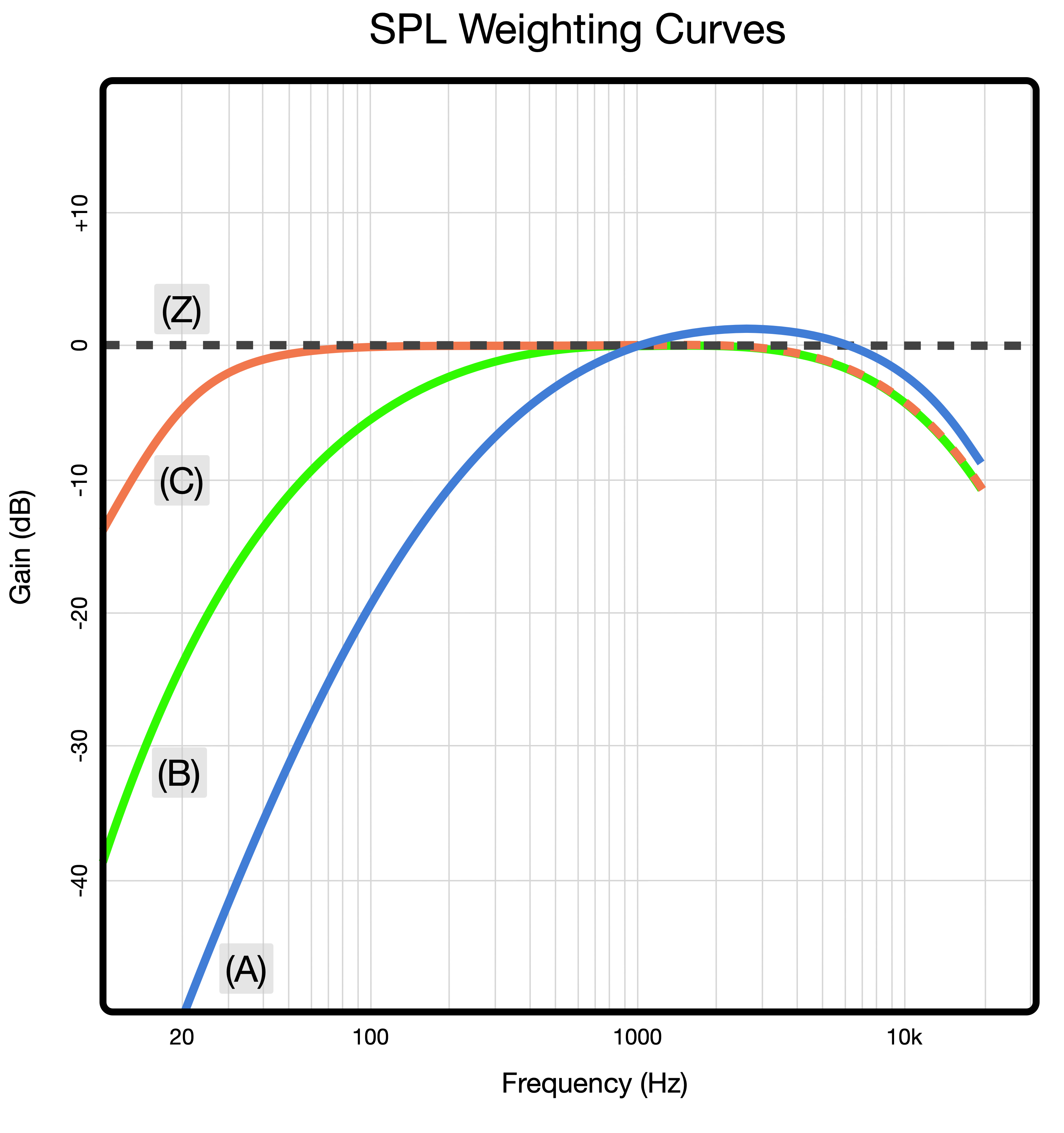
Weighting Curves – A, B, C, and Z
SPL tab parameters
Adjust the Project Settings parameters to change how pressure plots are displayed. Use the FILE > PROJECT SETTINGS menu (cmd-shift-P) and select the SPL tab to access these settings.

Project Settings – SPL Tab
SPL scaling
When SPL is selected, the average SPL (not peak) is represented by colors for the selected bandwidth. The default range and value settings can be changed by clicking the MANUAL buttons (above) and entering new values.
The Max Value is the loudest level plotted. If levels exceed this value, the area is plotted in white. Increase the Max Value until white is no longer displayed, see below.
The Min Range is the number of dB below the Max Value that will be plotted. If the prediction plane is plotted black, the SPL values are below the level range plotted. To plot as colors other than black, decrease the Max Value or increase the Min Range value, see below.

Model View – SPL, Change Only to Max Value Level: 85 dB (left), 100 dB (middle), and 115 dB (right)
When a loudspeaker is predicted with the Max Value = 75 dB, SPL values of 70 dB are plotted in red, (1) below. When the Max Value is set to 87 dB, 70 dB is plotted as yellow, (2) below. It’s the same data, just scaled and plotted differently.
For (2) below, when the Range = 42 dB, 42 dB of attenuation below the Max Value of 87 dB is plotted. In (3) below, when the Range = 30 dB, levels between 87 dB and 57 dB are plotted. 70 dB is now plotted as a light blue color. Again, it is the same data, just scaled and displayed differently.

Model View Predictions, SPL Mode – Same Data Represented Differently Based on SPL Max Level and Min Range Settings
The SPL values are only for the range of frequencies selected. When narrower prediction bandwidths are selected, the SPL values decrease. The pressure plots below use the same parameters for the same loudspeaker, the only change is the bandwidth of the prediction.

Model View, SPL – Less SPL as Bandwidth Narrows
Resolution
Resolution determines the number of colors used to represent pressure. Select Full Resolution, or level deviation per color used. The number of colors used to plot SPL or Attenuation can be helpful in different ways. Full Resolution uses a large number of colors to represent pressure, which are impressive images to include with a proposal. Using the 3 dB/color or 6 dB/color resolution settings makes determining coverage areas more obvious.
When changing between resolutions, no re-calculation is performed, the application only re-renders the prediction data.

Model View – Resolution Settings, Full Resolution, 0.5 dB, 1 dB, 3 dB, and 6dB Per Color
Attenuation range
The Attenuation selection uses colors to represent attenuation, normalized to the point on all of the prediction planes that has the highest pressure level. The color at the top of the scale (0 dB) represents this point. All other points are equal or less in level, represented by colors indicating level of attenuation.
To modify the range of SPL represented, click MANUAL and enter a higher or lower range of attenuation to display. This is the level of attenuation from 0 dB that will be plotted.

Model View – Attenuation, Min Range 42 dB, 30 dB, and 18dB
Attenuation examples
When using Attenuation mode, the level is relative to the loudest source. It is not intuitive that a subwoofer predicted at one-octave, 4 kHz appears to be very loud (below). It is in fact 30-40 dB lower in level at 4 kHz than within its operating range. Because the subwoofer is the loudest source in the model at this range of frequencies, the 0 dB color is plotted nearest this loudspeaker.

Model View – Subwoofer Prediction, One-Octave, 4 kHz
If a small, full-range loudspeaker (MM-4XP) is added to the model, the 0 dB color is plotted nearest the full-range loudspeaker because it is much louder than the subwoofer at 4 kHz.

Model View – Subwoofer and Mid-High Loudspeaker Prediction, One-Octave, 4 kHz
Appearance tab parameters
Adjust the Project Settings parameters to change how pressure plots are displayed. Use the PROJECT SETTINGS menu (cmd-shift-P) and select the APPEARANCE tab to access these settings.

Project Settings – Appearance Tab, Mesh Density and Pressure Map Opacity
Mesh density
The Mesh Density selection determines the resolution of the SPL map, and affects both calculation time and how detailed the pressure plot will be. A higher density has more points on the listening planes, creating a highly detailed pressure plot that takes longer to calculate than lower mesh densities (see below).

Model View Prediction – Mesh Density Setting Very Low (left), Very High (right)
Pressure Map opacity
Pressure Map Opacity changes the opacity of the prediction data in the Model View tab, 1.0 is opaque, 0.1 is almost transparent. (see below).

Model View – Pressure Map Opacity 1.0 and 0.7
Data Near Loudspeaker
Each loudspeaker data set has a small data void around the loudspeaker, intentionally.

Model View – Data Not Available Within One Meter
Example uses
Example 1: The Model View image below is of a one-octave, 4 kHz, 3 dB/color prediction. The colors indicate level on-axis , -3 dB down , -6 dB down for the octave centered at 4 kHz. When in SPL mode, the SPL values are for the bandwidth of the prediction only, one octave in this case. Relative pressure levels are available in Attenuation mode, the same as in MAPP XT.

Model View – One Octave, 4 kHz, 3 dB/Color, SPL Prediction – On-Axis (1), -3 dB (2), -6 dB (3)
Example 2: To evaluate coverage of a loudspeaker model using a standard level of variance for designs, +/- 3 dB or 6 dB, one option is to select Attenuation, Min Range = 12 dB. The first two colors indicate where coverage is within the design limits. The center of the red area is relative 0 dB. Between the red and yellow color is 3 dB less level. Between the yellow and green color is another 3 dB less level.

Model View – Attenuation, Range = 12 dB, Colors Represent Relative Level
Below, three different loudspeaker models are evaluated with slight location and aiming changes. On the left, the coverage is too narrow, even if the loudspeaker were better aimed. In the middle, there is too much level variation from front to rear. On the right, almost the entire half of the seating area is within 6 dB for the octave centered at 4 kHz. Fills may be necessary for rear of seating. For model selection, placement, and aiming, this viewing strategy is efficient.

Model View – Attenuation, Range = 12 dB, Evaluate Loudspeaker Location, Orientation, and Model Selection for Coverage
Measurement view
MAPP 3D provides two different methods to evaluate the performance of a system design:
The first is by showing sound pressure distribution over listening planes for a narrow range of frequencies—up to one octave wide—in the Model View tab. See Pressure plots.
The second is to add virtual microphones to the model in strategic locations to evaluate the broadband response and maximum acoustic output. This option is described below.
Analysis using only one of these methods is only partial analysis. Although it is true that most design work can be effectively accomplished using only Measurement View data, Model View predictions can inform microphone placement and help identify instances of coverage beyond the audience area(s).
To display prediction data in the Measurement View tab, at least one loudspeaker and one microphone must be added to the model.
Add microphones
Microphones are added to display broadband information and SPL values at the microphone locations.
INSERT > MICROPHONE or right-click in model, select INSERT MICROPHONE.
Use a Z-axis value representative of an average ear height.
Once inserted, microphones can be moved, copied, arrayed, mirrored, etc., in the same ways the geometry and loudspeakers are modified.
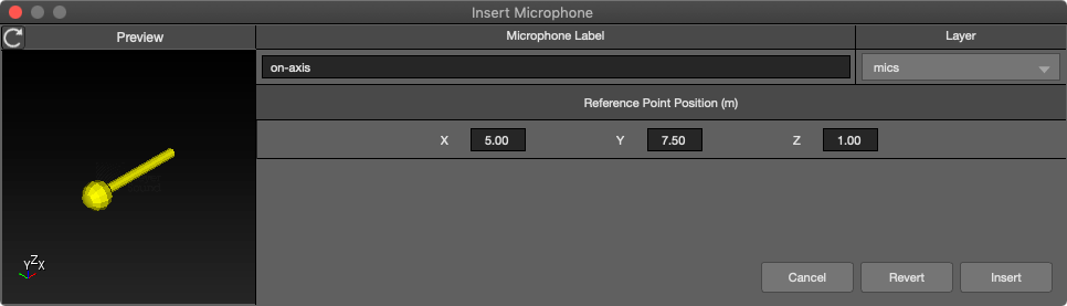
Insert Microphone Window
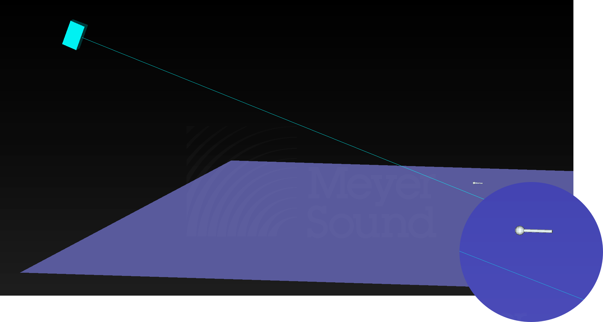
Model View – Microphone with Loudspeaker and Geometry
Microphone placement
There are many ways to approach system design and optimization; some provide more repeatable and homogeneous coverage results than others. Microphone placement is driven by design and optimization methodology. Below are some typical microphone placement methods.
Line Arrays: Generally, microphones are placed incrementally on-axis of a line array, at least at the beginning, middle, and end of coverage. For deeper coverage areas, additional microphones are placed incrementally.
Point Source Arrays: Generally, microphones are placed on-axis to the first element, at the -6 dB point1 of the first element, and on-axis of the adjacent array element.
Fills: Generally, on-axis to the larger system, at the -6 dB point1 of the larger system, and on-axis to the fill loudspeaker.
Note
1Within the range of frequencies that are directional, usually reproduced by a horn, generally 2 kHz to 20 kHz.
Frequency and IFFT response (SIM)
The Measurement View tab is based on the architecture and nomenclature of Meyer Sound’s SIM dual-channel FFT measurement platform, which is used in our anachoic chamber to collect data for MAPP 3D.
Frequency and IFFT response (SIM) tab overview
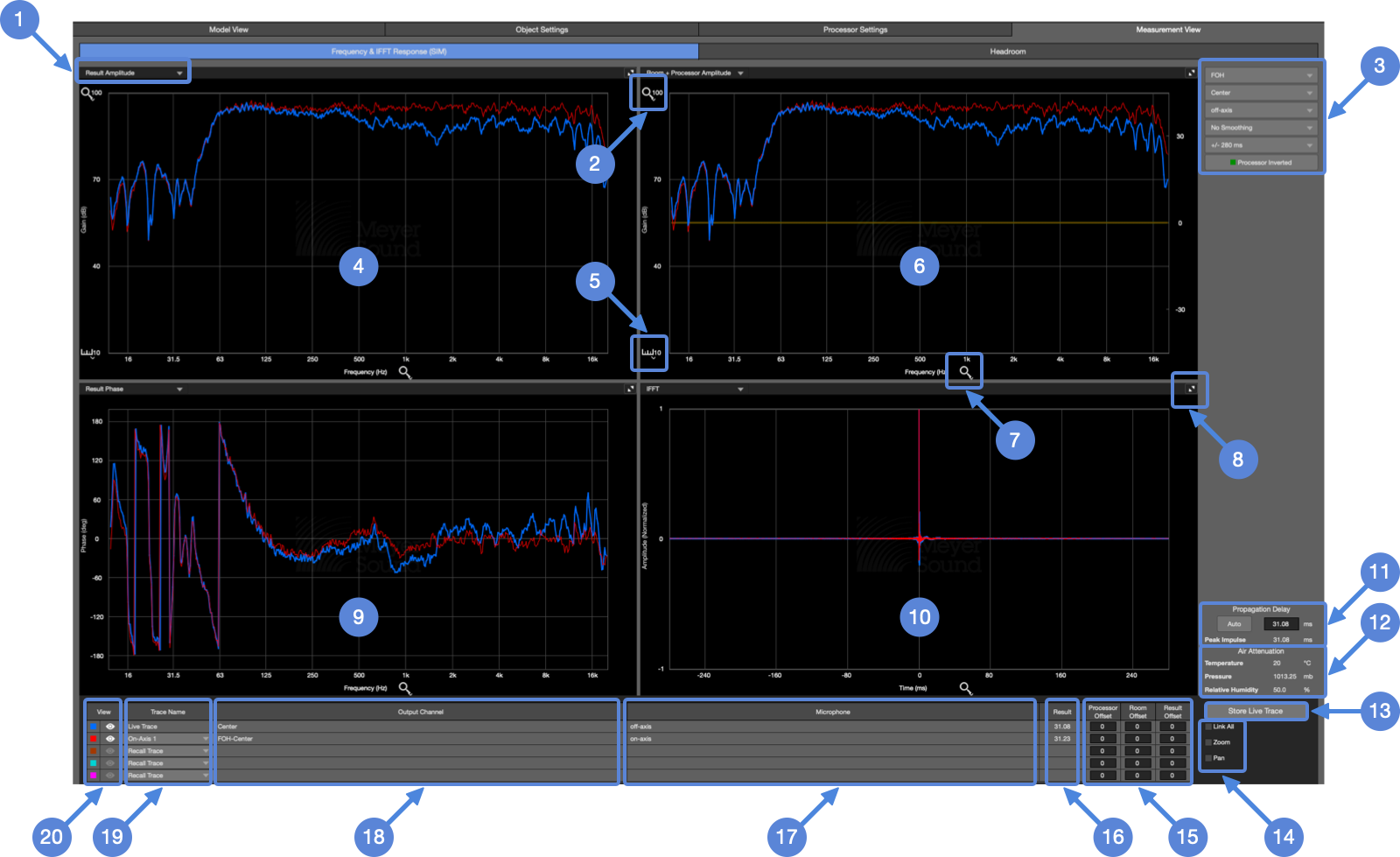
Measurement View Tab – Frequency & IFFT Tab
Plotter View Selection for each of the four panes, see options below this list
Zoom tool for vertical scale
Measurement Selection for processor, processor channel, microphone, smoothing level, IFFT window time, and processor trace toggle
Result Amplitude selected for this plotter
Vertical Scale dB/division selector
Room + Processor Amplitude selected for this plotter
Horizontal Zoom for each plotter
Expand/Collapse Plotter to occupy entire window
Result Phase response selected for this plotter
IFFT impulse response selected for this plotter
Propagation Delay amount of delay added to generator signal to synchronize with microphone
Air Attenuation current settings
Store Live Trace and name it for later recall—stores both the Headroom and Frequency & IFFT traces
Visual Options select to zoom and pan plotter view, link to zoom/pan like plotters
Trace Level Offset entered in dB
Propagation Delay for associated trace
Microphone name selected for live/stored trace
Processor Output Channel active for live/stored trace
Trace Recall drop-down to select stored traces
Show/Hide and Color selection for traces
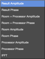
Measurement View – Frequency & IFFT, Pane View Selection Options
Frequency & IFFT response (SIM) signal patching
A transfer function is the difference between two signals. In order to compare them, the signals compared must be synchronized. Delay is added to the generator signal and to the processor signal to synchronize them with the microphone signal. This delay is added in MAPP 3D by clicking the Propagation Delay AUTO button. The delay time is displayed next to the AUTO button. A delay time can also be manually entered here.
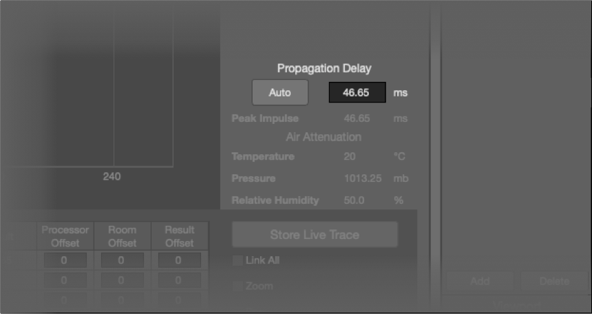
Measurement View, Frequency & IFFT Response Tab – Auto Propagation Delay
Three transfer functions are available: Processor, Speaker+Room, and Result, which are depicted below and used in MAPP 3D.
Note
In MAPP 3D, “Room” is the same as “Speaker + Room” used below.
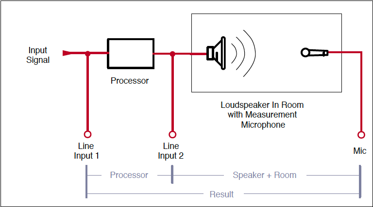
SIM Signal Patching and Transfer Function Names
For devices (processors and loudspeakers) that have the same performance at low and high levels, the transfer functions do not change for broadband, high density (not sparse) signals like pink noise, B-Noise, and M-Noise, which are selectable as the generator signal in MAPP 3D. The loudspeaker data sets in MAPP 3D are stored at the onset of limiting, the boundary of linear operation, which we use as the definition of maximum acoustic output.
The views available in the Frequency Response & IFFT panes are (defaults in bold):
Result Amplitude: the amplitude transfer function between the processor input and the microphone
Result Phase: the phase transfer function between the processor input and the microphone
Room Amplitude: the amplitude transfer function between the processor output and the microphone
Room Phase: the phase transfer function between the processor output and the microphone
Processor Amplitude: the amplitude transfer function between the input and output of the processor
Processor Phase: the phase transfer function between the input and output of the processor
Room + Processor Amplitude: the Room and Processor amplitude transfer functions displayed in the same plot
Room + Processor Phase: the Room and Processor phase transfer functions displayed in the same plot
IFFT: the Inverse Fast Fourier Transform, or the impulse response. Only available as the difference between source and the microphone (Result), which includes the processor, loudspeaker, and air propagation time.
Frequency and IFFT data usage
Observe the Result Amplitude trace as equalization and level adjustments are made if there is a target system response curve. The Result curve represents the spectral balance difference between the processor input and the loudspeaker output. If the Result trace is equal amplitude (flat), the system response will represent the input without changing the spectral balance. The proper spectral balance of a system is variable, usually based on a specification or a user’s expectation. It should be determined what the desired spectral balance of system is before committing to a design. Ensure the design has enough available headroom to reproduce the spectral content at the desired or specified level without exceeding available headroom.
Observe the Room + Processor Amplitude with the processor inverted for more precise equalization. Adjust equalization filters to match the inverted Processor trace to the Room trace; the Result will be equal amplitude (flat). It is not recommended to make equalization choices from only one microphone location for most applications. One exception would be a small control or listening room where there is only one primary listener.
Use the IFFT to synchronize arrivals of different sources:
measure, synchronize, and store the trace of the source that arrives latest in time
recall this trace (lower-left of window under Trace Name)
mute the first source, unmute the second source
click the AUTO button
The difference between the stored Propagation Delay (listed in the stored trace under Result) and the current Propagation Delay is the delay time to enter in the processor channel for the earlier arriving source to synchronize the two sources.
Signal generator
The generator level and signal type affect the SPL results.
The generator level is adjustable between -90 dB and +50 dB.
The generator signals available are:
Pink Noise: AES standard pink noise, broadband, with a crest factor of 12.5 dB (peak‑to‑RMS), in accordance with Audio Engineering Society loudspeaker test standards.
B‑Noise is band‑limited pink noise with a B-Weighed curve and increased crest factor, as defined in IEC 60268‑5 loudspeaker power testing practice.
Music‑Noise, as specified in AES75‑2023, is a standardized test signal with frequency‑dependent crest factor designed to emulate the dynamic characteristics of music program material. For more information, see aes.org/standards/AES75.
Weighting Curves – A, B, C, and Z
View options
Click-drag in any pane to display horizontal and vertical axis values.
Select ENABLE WINDOW CENTERING to vertically center amplitude plots.
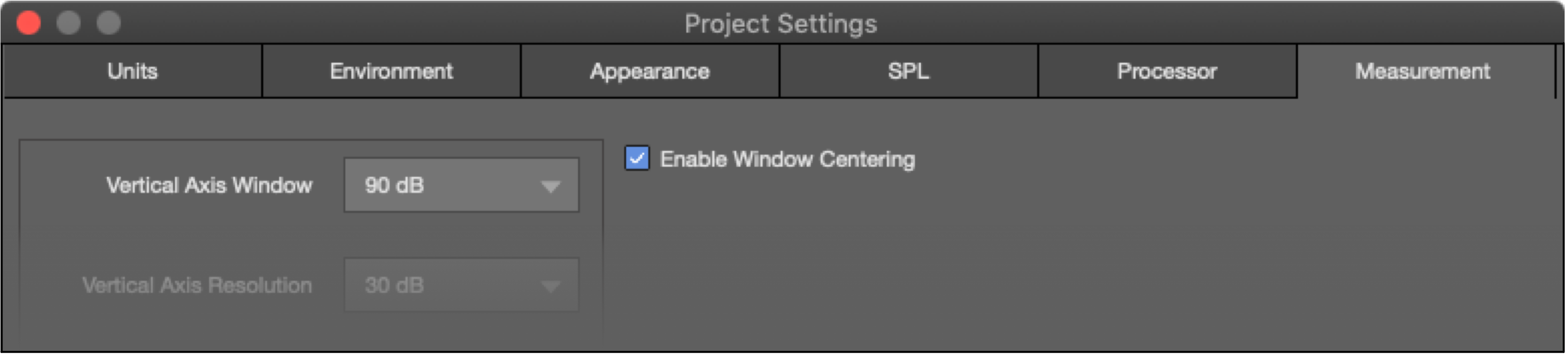
Select Enable Window Centering to Plot Traces at Vertical Center
The LINK ALL option links the Zoom and Pan settings for all like traces. All amplitude plots will have their Zoom/Pan settings linked. All phase plots will have their Zoom/Pan settings linked.
Zoom enables the use of the mouse wheel to zoom in/out of any pane.
Pan enables click-drag panning within a pane to view the entire plot when zoomed in.
Trace display
Up to five traces can be displayed in the data plots at the same time: the live trace and four previously stored traces. Each trace will be identified by the selected Output Channel, Microphone, and Propagation Delay. Enter offset values in dB for any trace.
Trace management
TOOLS > TRACE MANAGEMENT
Traces can be deleted by opening the Trace Management window from the Tools drop-down menu. Select the trace(s) to delete, click DELETE. When traces are stored, both the Frequency & IFFT and the Headroom data is stored using one name.
Headroom tab overview
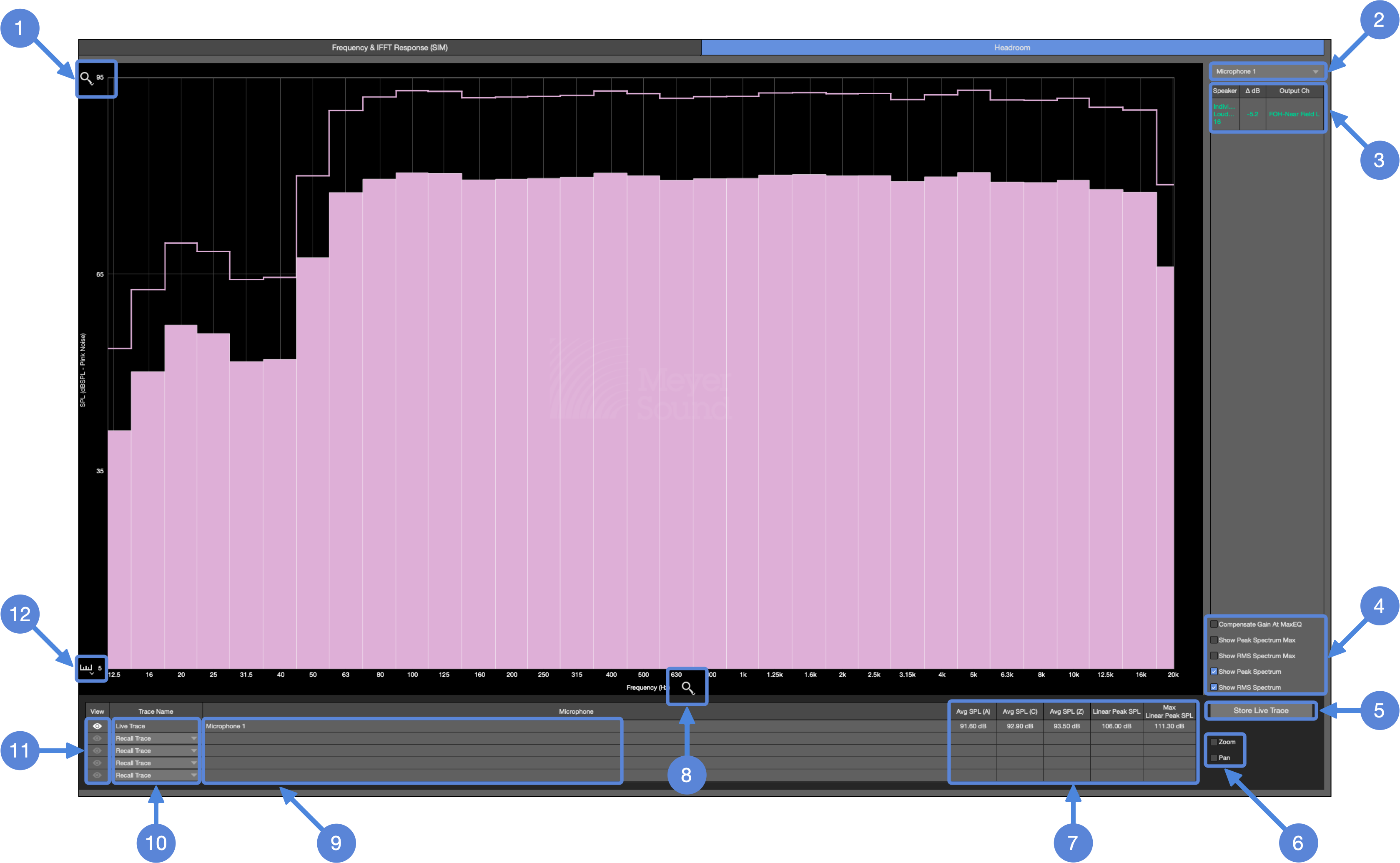
Measurement View Tab – Headroom Tab
Vertical Zoom of dBSPL axis
Microphone Selection for live trace
Headroom for Individual Loudspeakers remaining(+) or exceeded(-), relative to maximum linear output
Trace Toggles show/hide different plotter data, see below
Store Live Trace stores both the Headroom and Frequency & IFFT traces
Visual Options select to zoom and pan plotter view
SPL Values maximum SPL, dependent on generator signal type and level
Horizontal Zoom of plotter pane
Microphone name selected for live/stored trace
Trace Recall Selection drop-down to select stored traces
Show/Hide corresponding trace
Vertical Scale dB/division selector
Trace toggles
Make selections to show/hide available traces.
Show Peak Spectrum
Show RMS Spectrum
SPL values
The SPL values are dependent on signal generator level and signal type selected.
Average SPL (A-weighted) – broadband pink noise or B-Noise value
Average SPL (C-weighted) – broadband pink noise or B-Noise value
Average SPL (Z-no weighting) – broadband pink noise, B-Noise or M-Noise value
Linear Peak SPL – broadband pink noise, B-Noise or M-Noise value
Max Linear Peak SPL – ultimate broadband peak SPL that can be achieved if all elements of the system are phase-matched and time-aligned to the microphone position. This is a static value, unchanged by Generator level adjustments or processor output gain adjustments. While this is not a realistic operational level, it is helpful when determining whether a loudspeaker system is capable of achieving a specified SPL value.
Headroom data
The Headroom tab is used to determine the maximum SPL by 1/3 octave band and broadband output. This measurement is a single ended measurement, not a transfer function. Selecting different generator levels and signals will affect the SPL results. The available headroom for each loudspeaker of the system is listed (3 above).
The data in the plotter changes color depending on which signal generator choice is made:
Pink – Pink Noise
Blue – B-Noise
Yellow – M-Noise
Trace display
Up to five traces can be displayed in the data plots at the same time: the live trace and four previously stored traces. Each trace will be identified by the selected Output Channel, Microphone, and Propagation Delay. Enter offset values in dB for any trace.
Trace management
TOOLS > TRACE MANAGEMENT
Traces can be deleted by opening the Trace Management window from the Tools drop-down menu. Select the trace(s) to delete, click DELETE. When traces are stored, both the Frequency & IFFT and the Headroom data is stored using one name.
MAPP 3D SPL vs. product datasheet SPL
The data presented in MAPP 3D matches real-world measurements and our datasheets. However, comparisons need to be completed in a manner that is representative of the loudspeaker to microphone distance and the acoustic environment. Meyer Sound Laboratories typically lists Linear Peak SPL on the product datasheets for broadband models as:
measured in free-field at 4 m, referred to 1 m. Loudspeaker SPL compression measured with M-noise at the onset of limiting, 2-hour duration, and 50-degree C ambient temperature is < 2 dB.
For subwoofers, the product data sheet typically lists Linear Peak SPL as:
measured in half-space at 4 m referred to 1 m. Loudspeaker SPL compression measured with M-noise at the onset of limiting, 2-hour duration, and 50-degree C ambient temperature is < 2 dB.
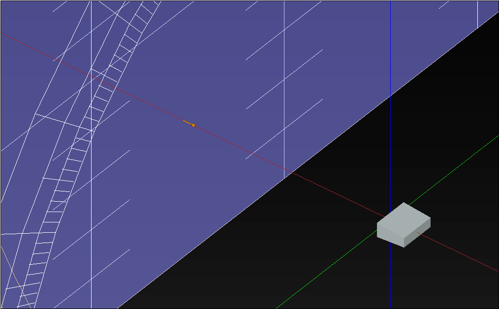
MAPP 3D, Lab 1.0 HR Project – Loudspeaker Face at 0 m ,0 m, 0 m, Microphone at 4 m, 0 m, 0 m
When loudspeaker data sets are acquired in our anachoic chamber, the distance between the loudspeaker and microphone is 4 meters. But, the industry typically specifies maximum SPL at a 1 meter distance. To convert a free-field, 4 meter test result to a 1 meter test result, the inverse square law is applied* and +12 dB is added to the result of the 4 meter test in free-field. This SPL value is listed on the loudspeaker data sheet making comparison to other 1 meter specifications simple.
For comparison of half-space, 1 meter measurements, where both the microphone and loudspeaker are on the ground, sound is radiated in one-half the area of the free-field measurement. Another +6 dB SPL is added because the radiation area is halved. Add +18 dB SPL to the result of a 4 meter, free-field measurement to compare it to a 1 meter, ground plane measurement.
To replicate this example in MAPP 3D:
open the Template Lab 1.0 HR (FILE > OPEN TEMPLATE)
move the microphone to 4 m, 0 m, 0 m (x, y, z coordinates)
place the loudspeaker face at 0 m, 0 m, 0 m (x, y, z coordinates)
predict using any of the noise sources
free-field: add +12 dB to the predicted Max Linear Peak SPL value in MAPP 3D
half-space: add +18 dB to the predicted Max Linear Peak SPL value in MAPP 3D
This result matches the Linear Peak SPL listed on the product datasheet.
* When the distance from a sound source is doubled, -6 dB SPL is lost. When the distance is halved, +6 dB SPL is gained. In this instance, 4 meters halved is 2 meters, and +6 dB SPL is gained. When 2 meters is halved, another +6 dB SPL is gained. In free-space, the SPL difference between a 4 meter measurement and a 1 meter measurement is +12 dB SPL.
Export documents
Various types of project information can be exported from MAPP 3D. Most are found in the FILE > EXPORT menu.
Model view screenshot
Exports a screenshot of the Model View. Select PNG or JPEG and Resolution, enter file name and select directory to save.
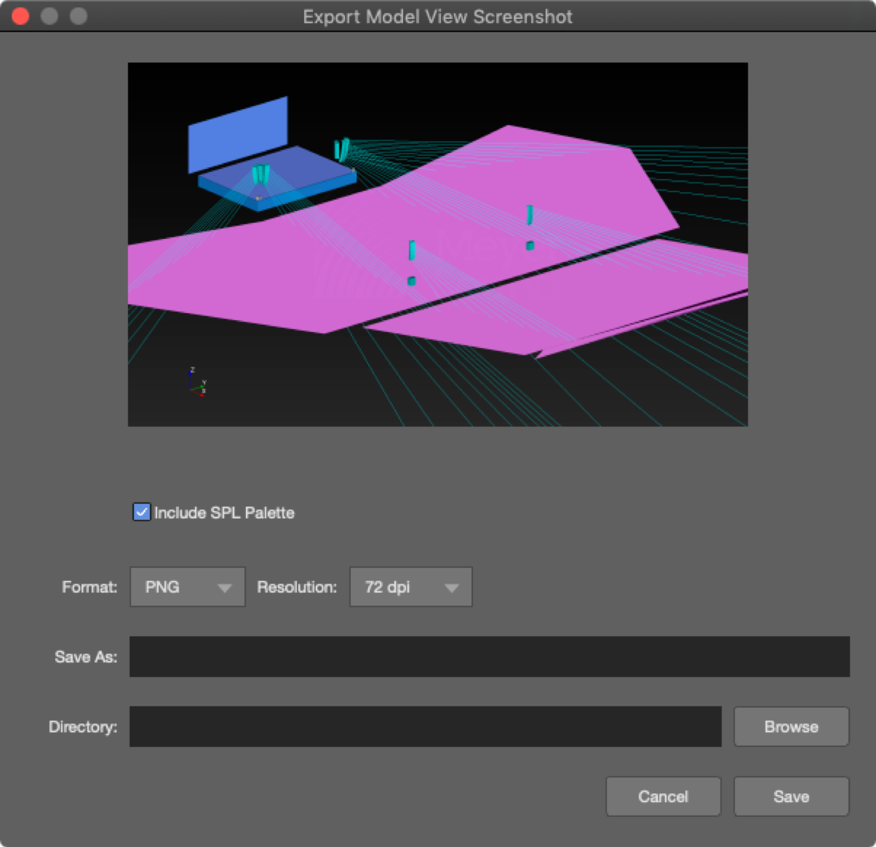
Export Model View Screenshot Dialog
Measurement view screenshot
Exports a screenshot of the Frequency & IFFT or Headroom, whichever is selected. Select PNG or JPEG and Resolution, enter file name and select directory to save.
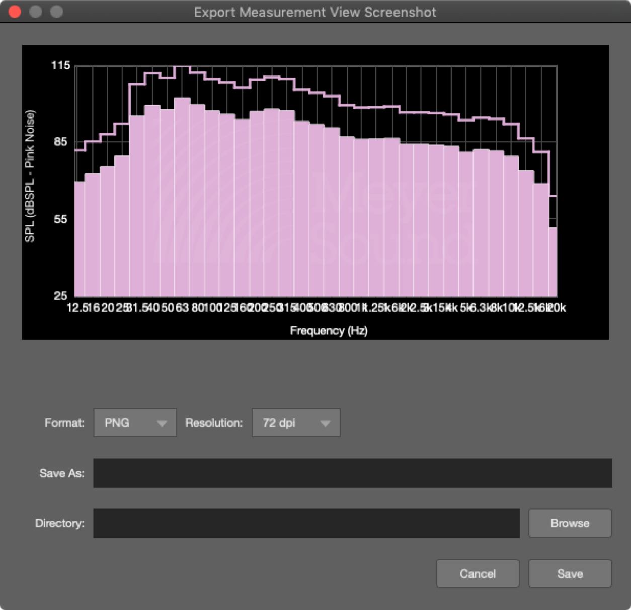
Export Measurement View Screenshot Dialog
Microphone data
Exports an XLS file that includes detailed information of every virtual microphone in the project.
Inventory to Excel
Exports an XLS file listing all of the hardware included in a project, e.g., loudspeakers, rigging hardware, and processors.
Processor patch list
Exports a PDF of the signal processing patch list for each processor in the project.
Export model view DXF
Exports a DXF file that includes all of the loudspeakers in the project drawn and positioned using the coordinate system of the MAPP3D project. This is useful for integrating MAPP 3D designs with external documentation for the project or application.
Loudspeaker system report
Select a loudspeaker or loudspeaker system in Model View, right-click, and select Loudspeaker System Report. A detailed report is created. Click GENERATE to save the PDF.
More
All settings and preferences
This section provides the complete list of settings and preferences available in the MAPP 3D application.
Project settings
FILE > PROJECT SETTINGS Parameters in this window define the workspace and how the application presents data.
Units
Select the preferred unit of measure for each of the listed parameters.
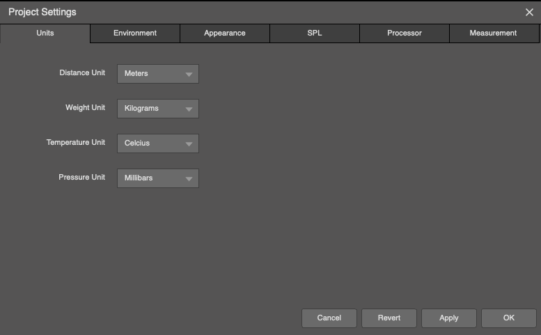
Project Settings – Units
Environment
Temperature, humidity, and altitude settings are used to model high-frequency loss due to air absorption. Select USE AIR ATTENUATION (on by default) to include this feature when predicting.
The source voltage, which affects the current draw estimates, is selected here. Voltage selection can also be changed using the drop-down in the main application window.
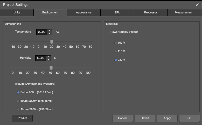
Project Settings – Environment
Appearance
Set Axis Limits boundary limits (size) of the workspace in Model View. These settings control the maximum/minimum XYZ coordinates of the Model. Objects cannot be placed outside of the defined space.
Mesh Density determines the resolution of the SPL map and affects both calculation time and how detailed the map will be. A higher density will ‘sample’ more points on the listening planes, which takes longer and creates a highly detailed pressure plot.
Select Color Scheme as White for better viewing outdoors.
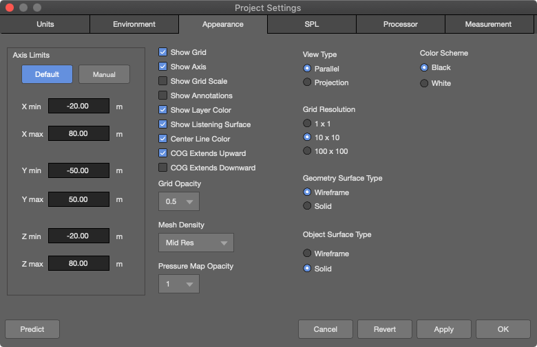
Project Settings – Appearance
SPL
When SPL units are selected, absolute SPL values within the selected range (e.g., for one octave, centered at 4 kHz) will be plotted on the listening planes. When Attenuation is selected, levels will be displayed as relative attenuation from the loudest sound source (similar to MAPP XT). Resolution determines how SPL maps are displayed—full resolution, or various increments in level with each color change.
This tab can also be accessed directly by right-clicking in Model View and selecting Set Max SPL.
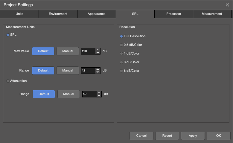
Project Settings – SPL
Processor
When selected, Atmos. Corr. Response enables the display of the compensation filters in the Processor Settings tab used to correct for high-frequency air absorption.
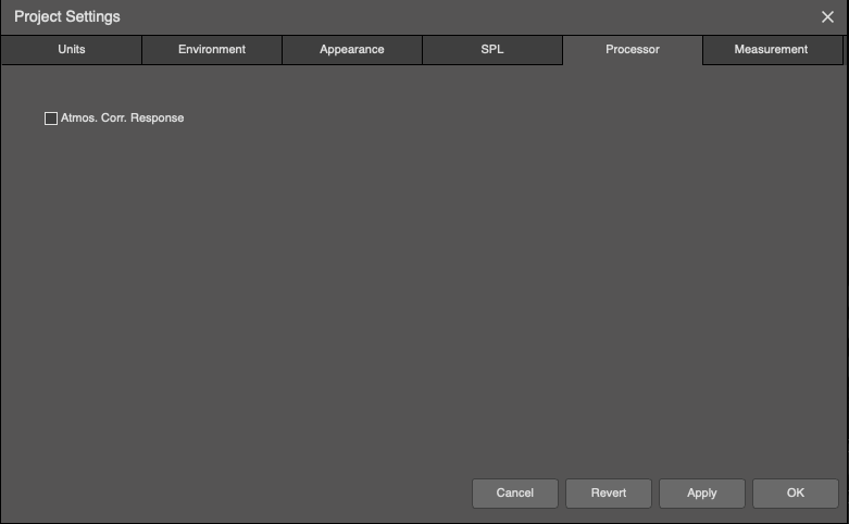
Project Settings – Processor
Measurement
These preferences change the plotting scales in the Measurement View tab. These parameters can also be changed in the Measurement View tab by clicking icons next to the plotters.
Select ENABLE WINDOW CENTERING to vertically center amplitude plots.
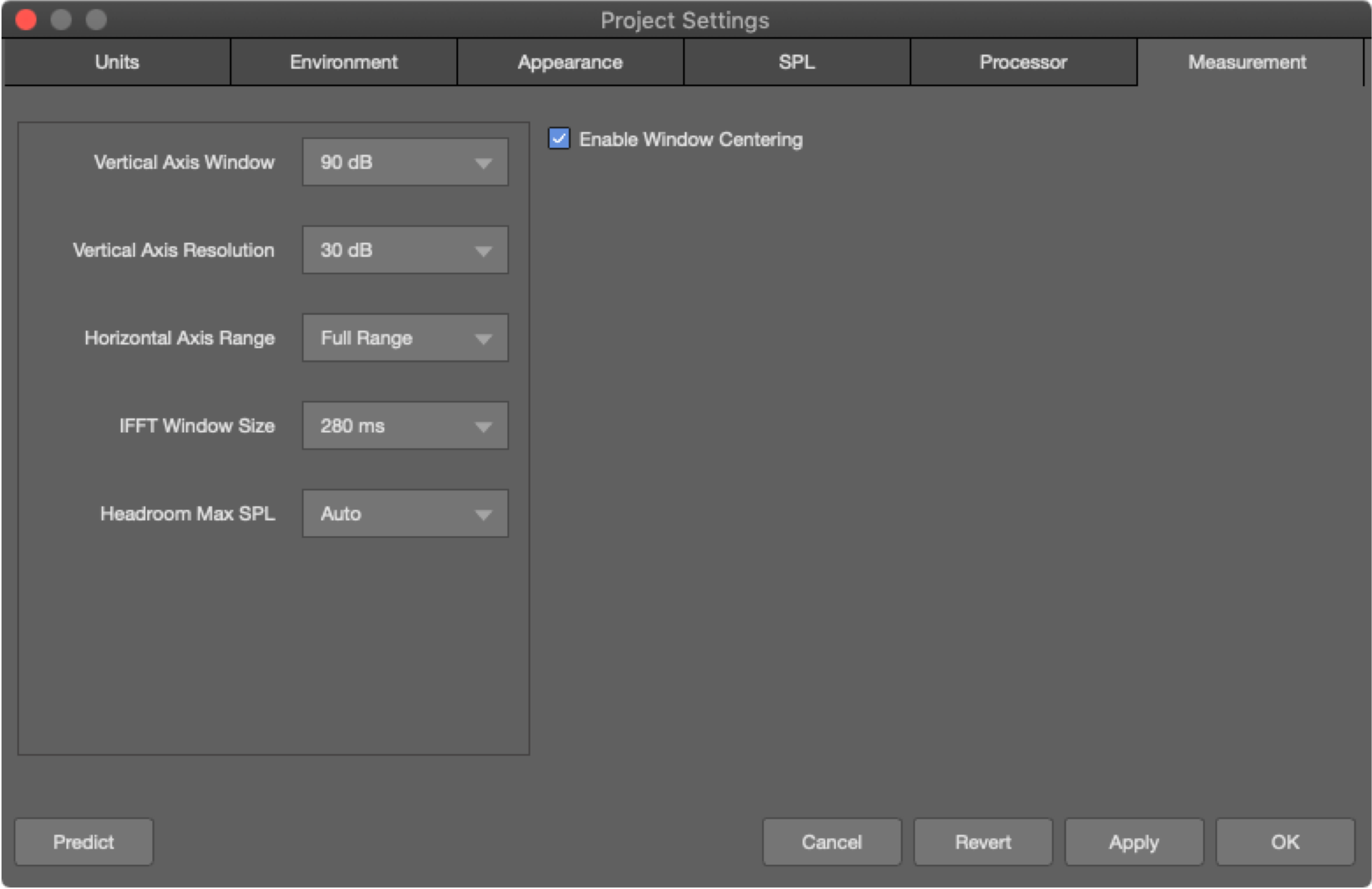
Project Settings – Measurement
View menu
Use the View menu to choose optional items shown in the Model View tab. Click on an item to toggle on/off.
View Menu
Center lines
Center Lines indicate the direction a loudspeaker is pointing. This is the global control. Each loudspeaker or loudspeaker array also has a center line preference, changed either in the Express Settings tab or Object Settings tab.
Geometry has a preference for Through. When selected, the center lines will go through the geometry. If not selected, the center line will terminate at the geometry. This is useful to determine if there is line of site between a loudspeaker and a seating area (for example, under-balcony seating).
Center Lines Selected, Balcony Not Selected Through, Orchestra Selected Through
Center of gravity (COG)
When selected, Center of Gravity (COG) turns on the indicator in Model View. Used to determine minimum/maximum uptilt or downtilt of array grids. Used to determine which center pick-up point to use to achieve a specific up/downtilt of grids with center pick-up bars. Select array to view intersection of COG marker and rigging holes of center bar.
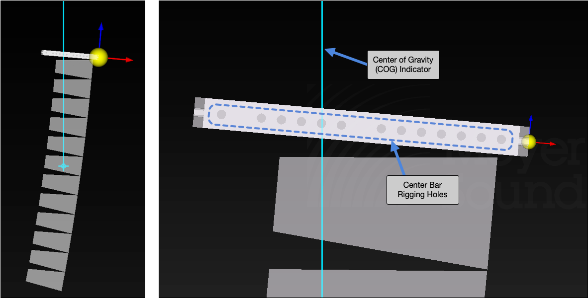
Center of Gravity Indicator
Base marker
For loudspeaker arrays in Model View, the Base Marker indicates the point on the vertical axis (Z) of an array closest to the Z plane (usually the floor or ground).
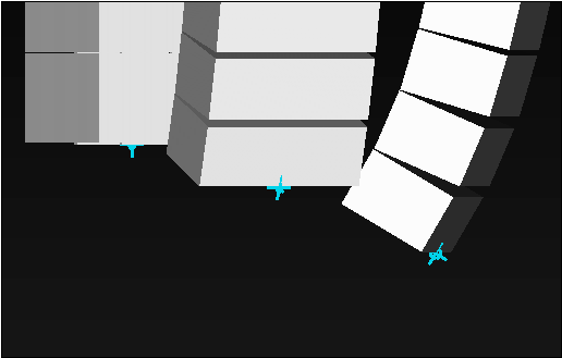
Base Marker Indicator
Front / rear rig point marker
When selected, indicates the front and/or rear rigging point of a grid used to suspend a flown loudspeaker array.
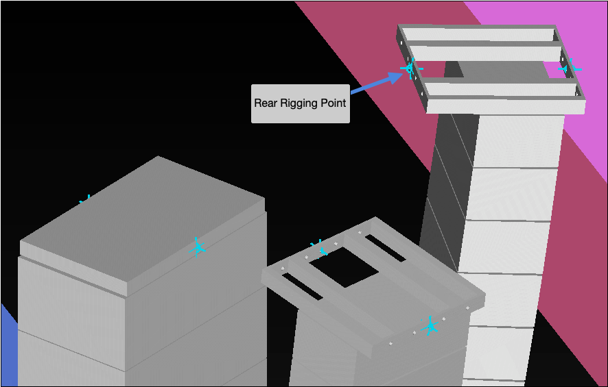
Front and Rear Rigging Point Indicators
Grid
In Model View, toggles reference grid on/off. Also found in FILE > PROJECT SETTINGS, Appearance tab: with Resolution, Scale, and Opacity preferences
Grid scale
In Model View, toggles numeric labeling of grid lines at boundary of pane. Also found in FILE > PROJECT SETTINGS, Appearance tab
Grid Scale
Zoom to extents
In Model View, zooms to include all objects in the model.
Perspective view
By default, Model View displays a parallel view. Zoom in/out when in top, bottom, left or right views does not change the appearance. For a more 3D view, select Perspective. When zoomed in/out, the appearance is similar to that of reality.
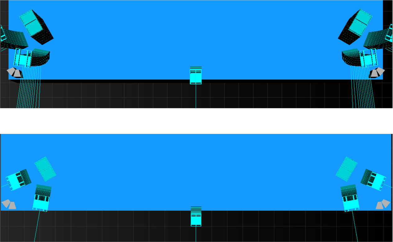
Model View – Perspective View (top), default Parallel View (bottom)
Camera points
Displays the camera locations for cameras that have viewpoints within the axis limits, shown as grey pyramids. The default camera views are not displayed. User created cameras are displayed.
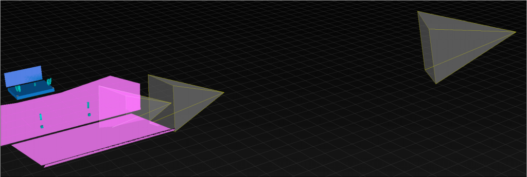
Model View – Three Camera Points
Export overlay
Adds a highlight box to the Model View tab to indicate the area of the window that will be exported. Select orientation and size from the sub-menu.
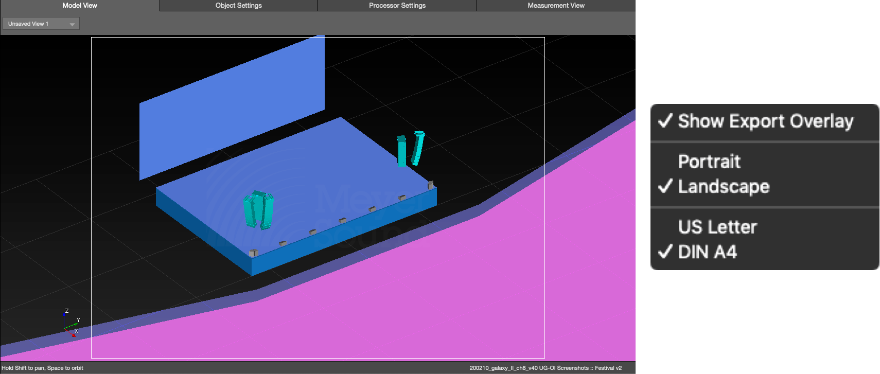
Model View – Export Overlay Selected